- What is object detection?
- How does object detection work?
- What is YOLO object detection?
- Overview of YOLO object detection algorithm
- Non-Maximum Suppression
- Implementation of YOLO with OpenCV
- Custom Object detection with YOLO
What is Object Detection?
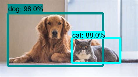
Object detection is a computer vision technique in which a software system can detect, locate, and trace the object from a given image or video. The special attribute about object detection is that it identifies the class of object (person, table, chair, etc.) and their location-specific coordinates in the given image. The location is pointed out by drawing a bounding box around the object. The bounding box may or may not accurately locate the position of the object. The ability to locate the object inside an image defines the performance of the algorithm used for detection. Face detection is one of the examples of object detection.
These object detection algorithms might be pre-trained or can be trained from scratch. In most use cases, we use pre-trained weights from pre-trained models and then fine-tune them as per our requirements and different use cases.
How does Object Detection work?
In this section, we will briefly go through the different approaches that are taken in Object detection tasks. There are two approaches to Object detection and they are:
- Two-shot detection.
- Single-shot detection.
Let us first find about Two-shot detection method. As the name suggests there are two stages involved in this method. One is region proposal and then in the second stage, the classification of those regions and refinement of the location prediction takes place.
Faster-RCNN variants are the popular choice of usage for two-shot models. Here during the region proposal stage, we use a network such as ResNet50 as a feature extractor. We do this by removing the last layers of this network and just use the rest of the layers to extract features from the images. This is usually a better approach as the network is already trained and can extract features from the images. Next, a small fully connected network slides over the feature layer to predict class-agnostic box proposals, with respect to a grid of anchors tiled in space, scale and aspect ratio.
In the second stage, these box proposals are used to crop features from the intermediate feature map which was already computed in the first stage. The proposed boxes are fed to the remainder of the feature extractor in which the prediction and regression heads are added on top of the network. Finally, in the output, we get the class and class-specific box refinement for each proposal box.
On the contrary side, Single-shot detection skips the region proposal stage and yields final localization and content prediction at once.YOLO is a popular example of this approach and we are going to discuss the working of it in the coming sections.
It must be noted that two-shot detection models achieve better performance but single-shot detection is in the sweet spot of performance and speed/resources which makes it more suitable for tasks like detecting objects in live feed or object tracking where the speed of prediction is of more importance.
What is YOLO object detection?
As mentioned already, YOLO which stands for “You only look once” is a single shot detection algorithm which was introduced by Joseph Redmon in May 2016. Although the name of the algorithm may sound strange, it gives a perfect description of this algorithm as it predicts classes and bounding boxes for the whole image in one run of the algorithm.
YOLO performed surprisingly well as compared to the other single-shot detectors of that time in terms of speed and accuracy. It is not the most accurate algorithms when it comes to object detection but certainly, it makes that up with its impressive speed and thus is a good balance between speed and accuracy.
Overview of YOLO object detection algorithm
The YOLO network splits the input image into a grid of S×S cells. If the centre of the ground truth box falls into a cell, that cell is responsible for detecting the existence of that object.
Each grid cell predicts B number of bounding boxes and their objectness score along with their class predictions as follows:
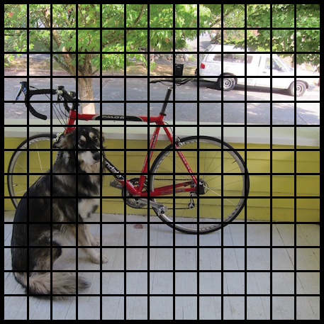
- Coordinates of B bounding boxes -YOLO predicts 4 coordinates for each bounding box (bx,by,bw,bh) with respect to the corresponding grid cell. Here bx, by are the x and y coordinates of the midpoint of the object with respect to this grid. The value of bh is the ratio of the height of the bounding box to the height of the corresponding grid cell and bw is the ratio of the width of the bounding box to the width of the grid cell.
- Objectness score (P0) – indicates the probability that the cell contains an object. The objectness score is passed through a sigmoid function to be treated as a probability with a value range between 0 and 1.
- Class prediction – if the bounding box contains an object, the network predicts the probability of K number of classes. Where K is the total number of classes in your problem.
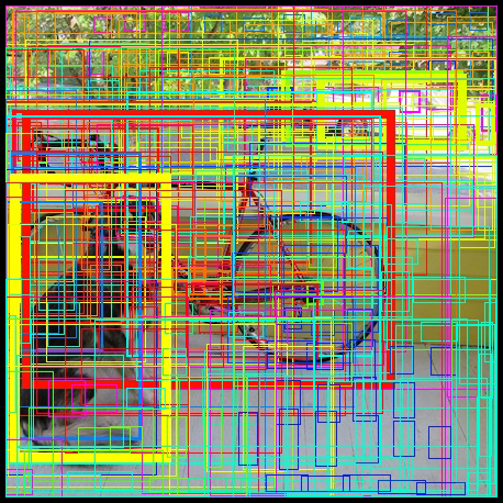
The predicted bounding boxes may look something like the following (the higher the confidence score, the fatter the box is drawn):
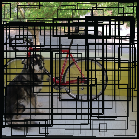
Finally, the confidence score for the bounding box and the class prediction are combined into one final score that tells us the probability that this bounding box contains a specific type of object. For example, the big fat yellow box on the left is quite sure it contains the object “dog”:
It turns out that most of these boxes will have very low confidence scores, so we only keep the boxes whose final score is above some threshold. Also, Non-maximum Suppression (NMS) intends to cure the problem of multiple detections of the same image. In the next section, we will briefly go over it. The final prediction is then:
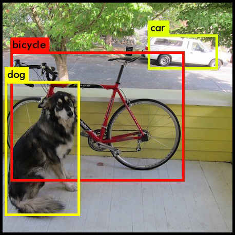
It is important to note that before v3, YOLO used softmax function for the class scores. In v3 the authors have decided to use sigmoid instead. The reason is that Softmax imposes the assumption that each box has exactly one class which is often not the case. In other words, if an object belongs to one class, then it’s guaranteed it cannot belong to another class. While this assumption is true for some datasets, it may not work when we have classes like Women and Person. A multilabel approach models the data more accurately. This is the reason that authors have steered clear of using a Softmax activation.
Non-maximum Suppression
Non-maximum Suppression or NMS uses the very important function called “Intersection over Union”, or IoU. Here is how we calculate IoU.

We define a box using its two corners (upper left and lower right): (x1, y1, x2, y2) rather than the midpoint and height/width. Next, we also need to find the coordinates (xi1, yi1, xi2, yi2) of the intersection of two boxes where :
xi1 = maximum of the x1 coordinates of the two boxes
yi1 = maximum of the y1 coordinates of the two boxes
xi2 = minimum of the x2 coordinates of the two boxes
yi2 = minimum of the y2 coordinates of the two boxes
Note that to calculate the area a rectangle (or a box) we can to multiply its height (y2 – y1) by its width (x2 – x1).
So to calculate IoU, first calculate the area of intersection by this formula
area_intersection =(xi2 - xi1)*(yi2 - yi1)
Next, calculate the area of union
union _area = (area of box 1 + area of box 2) - area_intersection
Therefore IoU=area_intersection/union_area
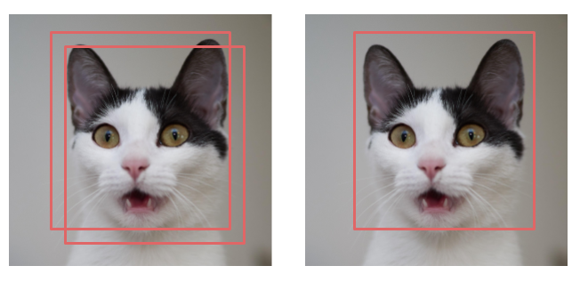
Now, to implement non-max suppression, the steps are:
- Select the box that has the highest score.
- Compute its overlap with all other boxes, and remove boxes that overlap it more than a certain threshold which we call iou_threshold.
- Go back to step 1 and iterate until there are no more boxes with a lower score than the currently selected box
These steps will remove all boxes that have a large overlap with the selected boxes. Only the best boxes remain.
Click here to see the Keras Implementation of YOLO algorithm
Implementation of YOLO with OpenCV
There are various implementations of YOLO algorithm and perhaps most popular of them is the Darknet. But here we are going to use OpenCV to implement YOLO algorithm as it is really simple. To get started you need to install OpenCV on your Pc using this command in you command prompt.
pip install opencv-pythonTo use YOLO via OpenCV, we need three files viz -’yoloV3.weights’, ‘yoloV3.cfg’ and “coco.names” ( contain all the names of the labels on which this model has been trained on).Click on them o download and then save the files in a single folder. Now open a python script in this folder and start coding:
First, we are going to load the model using the function “cv2.dnn.ReadNet()”.This function loads the network into memory and automatically detects configuration and framework based on file name specified.
import cv2
import numpy as np

# Load Yolo
print("LOADING YOLO")
net = cv2.dnn.readNet("yolov3.weights", "yolov31.cfg")
#save all the names in file o the list classes
classes = []
with open("coco.names", "r") as f:
    classes = [line.strip() for line in f.readlines()]
#get layers of the network
layer_names = net.getLayerNames()
#Determine the output layer names from the YOLO model
output_layers = [layer_names[i[0] - 1] for i in net.getUnconnectedOutLayers()]
print("YOLO LOADED")
After loading the model now either we can use it detects objects in an image or you can even use it for real-time object detection for which you are going to need a PC with good processing speed.
Here is the code to detect objects in images
 # Capture frame-by-frame
    img = cv2.imread("test_img.jpg")
#     img = cv2.resize(img, None, fx=0.4, fy=0.4)
    height, width, channels = img.shape

    # USing blob function of opencv to preprocess image
    blob = cv2.dnn.blobFromImage(img, 1 / 255.0, (416, 416),
     swapRB=True, crop=False)
    #Detecting objects
    net.setInput(blob)
    outs = net.forward(output_layers)

    # Showing informations on the screen
    class_ids = []
    confidences = []
    boxes = []
    for out in outs:
        for detection in out:
            scores = detection[5:]
            class_id = np.argmax(scores)
            confidence = scores[class_id]
            if confidence > 0.5:
                # Object detected
                center_x = int(detection[0] * width)
                center_y = int(detection[1] * height)
                w = int(detection[2] * width)
                h = int(detection[3] * height)

                # Rectangle coordinates
                x = int(center_x - w / 2)
                y = int(center_y - h / 2)

                boxes.append([x, y, w, h])
                confidences.append(float(confidence))
                class_ids.append(class_id)

    #We use NMS function in opencv to perform Non-maximum Suppression
    #we give it score threshold and nms threshold as arguments.
    indexes = cv2.dnn.NMSBoxes(boxes, confidences, 0.5, 0.4)
    colors = np.random.uniform(0, 255, size=(len(classes), 3))
    for i in range(len(boxes)):
        if i in indexes:
            x, y, w, h = boxes[i]
            label = str(classes[class_ids[i]])
            color = colors[class_ids[i]]
            cv2.rectangle(img, (x, y), (x + w, y + h), color, 2)
            cv2.putText(img, label, (x, y -5),cv2.FONT_HERSHEY_SIMPLEX,
			1/2, color, 2)

    cv2.imshow("Image",img)
    cv2.waitKey(0)
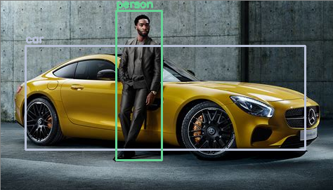
Output:

Click here to see the Keras Implementation of YOLO algorithm
Here is the code to detect objects in real-time using webcam
video_capture = cv2.VideoCapture(0)
while True:
    # Capture frame-by-frame
    re,img = video_capture.read()
    img = cv2.resize(img, None, fx=0.4, fy=0.4)
    height, width, channels = img.shape

    # USing blob function of opencv to preprocess image
    blob = cv2.dnn.blobFromImage(img, 1 / 255.0, (416, 416),
     swapRB=True, crop=False)
    #Detecting objects
    net.setInput(blob)
    outs = net.forward(output_layers)

    # Showing informations on the screen
    class_ids = []
    confidences = []
    boxes = []
    for out in outs:
        for detection in out:
            scores = detection[5:]
            class_id = np.argmax(scores)
            confidence = scores[class_id]
            if confidence > 0.5:
                # Object detected
                center_x = int(detection[0] * width)
                center_y = int(detection[1] * height)
                w = int(detection[2] * width)
                h = int(detection[3] * height)

                # Rectangle coordinates
                x = int(center_x - w / 2)
                y = int(center_y - h / 2)

                boxes.append([x, y, w, h])
                confidences.append(float(confidence))
                class_ids.append(class_id)

    #We use NMS function in opencv to perform Non-maximum Suppression
    #we give it score threshold and nms threshold as arguments.
    indexes = cv2.dnn.NMSBoxes(boxes, confidences, 0.5, 0.4)
    font = cv2.FONT_HERSHEY_PLAIN
    colors = np.random.uniform(0, 255, size=(len(classes), 3))
    for i in range(len(boxes)):
        if i in indexes:
            x, y, w, h = boxes[i]
            label = str(classes[class_ids[i]])
            color = colors[class_ids[i]]
            cv2.rectangle(img, (x, y), (x + w, y + h), color, 2)
            cv2.putText(img, label, (x, y + 30), font, 2, color, 3)

    cv2.imshow("Image",cv2.resize(img, (800,600)))
    if cv2.waitKey(1) & 0xFF == ord('q'):
        break
video_capture.release()
cv2.destroyAllWindows()
Real-time Object Detection Using TensorFlow object detection API
Custom Object detection with YOLO
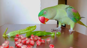
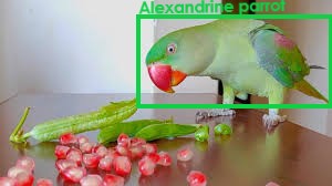
In this section, we will see how we can create our own custom YOLO object detection model which can detect objects according to our preference. Here I am going to show how we can detect a specific bird known as Alexandrine parrot using YOLO. Note that this model can only detect the parrot but we can train it to detect more than one object.
The first thing we need is images of parrots. We can download them manually from the internet but that is really slow and tiring. Alternatively, you can use tools which are freely available on GitHub. Here is one that you can use and you can find the instructions to use it from the same GitHub page. You need to download at least 300 images to get decent results.
Next, we need to manually label each image with the location of the parrots in the images. We can use a tool labelImg for this and it can make our work really easy but still it is going to take time as we have to do this manually. Remember to change the settings and keep it for YOLO as I will point out in the video below. Before moving forward make sure that all your images are in the same folder and the folder contains only the images we want.
Now zip the folder which contains all the images along with the .txt files containing the location of the object and upload them to your google drive. Also, make a folder in your drive by the name of yolov3 and place the zip file in that folder.
Next, open this Colab Notebook via your account and run all the cells. Be sure to change all the paths according to your files or you can change the name of the zip folder of your data to ‘logo’ as I have, and then you don’t need to change anything.
It may take around 5-6 hours before you can see your average loss touching 0.1 and then you can stop the training but interrupting the cell. You will see the new weights file in the yolov3 folder of your google drive.
Now all you need to do is modify the above code and you have your custom object detector. Just replace the weights with the new weights we got after training and just put one item i.e “Alexandrine parrot” in classes list.
This brings us to the end of this article where we learned what is YOLO and how can we can use OpenCV to implement YOLO. To get a free course on Computer vision, click the banner below.


