What is Predictive Modeling? Types and Functions

Ever been curious about how companies forecast sales, identify fraud, or suggest products you adore?

The answer is predictive modeling, a method that uses past data to forecast the future.

In this article, we’ll demystify the process of predictive modeling, see how it’s applied, and why it’s crucial in the data age.

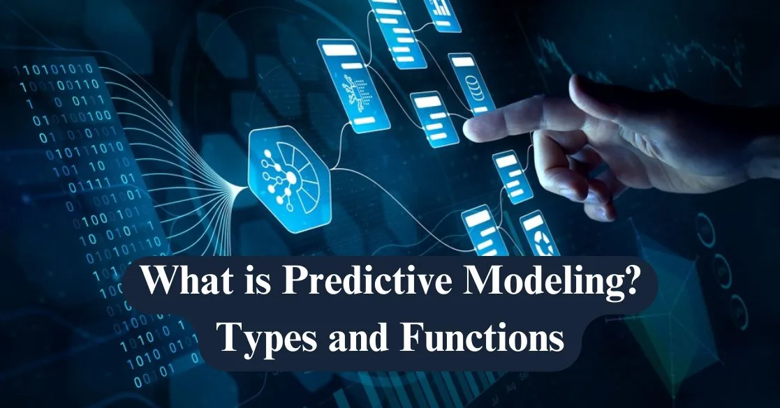
Definition of Predictive Modeling

Predictive modeling is a data-driven technique that uses statistical algorithms & machine learning methods to analyze historical data and predict future outcomes.

It assists businesses & organizations make informed decisions by identifying patterns, trends, and relationships within data.

Predictive models are widely used in industries like finance, healthcare, marketing, and cybersecurity to forecast risks, detect fraud, and optimize operations.

Key Components of Predictive Modeling

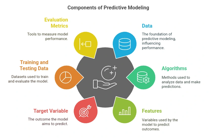
1. Data
   • The foundation of predictive modeling. It can be structured (numerical, categorical) or unstructured (text, images, audio).
   • The quality, diversity, and volume of data influence model performance.

Also Read: Types of Data

2. Algorithms
   • Different machine learning and statistical algorithms are used based on the problem type.
   • Examples include:
     • Linear Regression, Decision Trees, Random Forest, and Neural Networks for general predictive tasks.
     • Clustering algorithms (e.g., K-Means) for grouping similar data points.
     • Deep Learning models for complex tasks like image recognition.

3. Features (Predictors)
   • The independent variables or attributes used by the model to make predictions.
   • Example: In predicting customer churn, features may include transaction history, service complaints, and customer engagement metrics.

4. Target Variable
   • The dependent variable or the outcome that the model aims to predict.
   • Example: In fraud detection, the target variable could be binary (fraudulent or non-fraudulent transaction).

5. Training and Testing Data
   • The dataset is typically split into training (80%) and testing (20%) sets to assess model performance.
   • Cross-validation techniques, like k-fold validation, help ensure robustness.

6. Evaluation Metrics
   • Used to measure how well a model performs.
   • Examples:
     • AUC-ROC (Area Under Curve – Receiver Operating Characteristic) for classification models.
     • R-squared (R²) score for regression models.

7. Model Deployment & Feedback Loop
   • Once a model is deployed, it continuously learns from new data.
   • Periodic retraining ensures it adapts to changing patterns and improves accuracy over time.

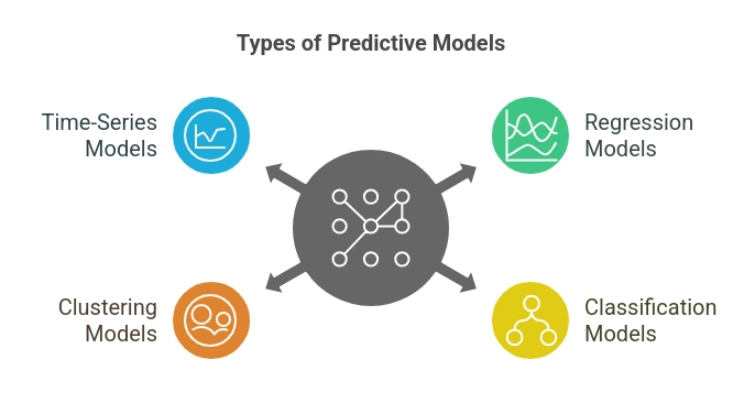
Types of Predictive Models

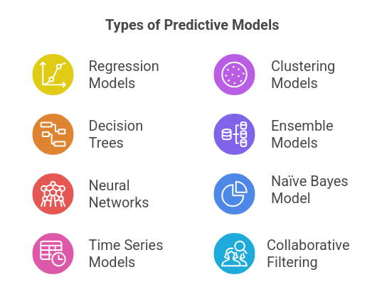
1. Regression Models

Regression models predict a continuous numeric value based on input variables. They are widely used in finance, economics, and sales forecasting.

• Linear Regression – Establishes a relationship between independent and dependent variables using a straight-line equation.
• Logistic Regression – Used for binary classification problems (e.g., predicting whether a customer will churn or not).
• Polynomial Regression – Models complex relationships using polynomial equations.
• Example: Predicting house prices based on features like location, size, and number of rooms.

2. Decision Trees

A decision tree is a tree-like model that splits data based on conditions at each node, making predictions based on a series of decisions.

• Classification and Regression Trees (CART) – Used for both classification and regression tasks.
• Random Forest – An ensemble of multiple decision trees that improves accuracy by reducing overfitting.
• Example: Predicting loan approval based on credit history and income level.

3. Neural Networks

Inspired by the human brain, neural networks are deep learning models capable of identifying complex patterns.

• Feedforward Neural Networks (FNNs) – Used for structured data analysis.
• Recurrent Neural Networks (RNNs) – Effective for sequential data, such as time series forecasting.
• Convolutional Neural Networks (CNNs) – Commonly used in image and video recognition.
• Example: Detecting fraudulent transactions by analyzing transaction patterns in banking.

4. Time Series Models

Time series models analyze sequential data to forecast future values based on past trends.

• ARIMA (AutoRegressive Integrated Moving Average) – Commonly used for economic and financial forecasting.
• LSTMs (Long Short-Term Memory Networks) – A type of RNN designed for long-term dependency tasks.
• Example: Forecasting stock prices or predicting weather conditions.

5. Clustering Models

Clustering models group similar data points together based on common characteristics.

• K-Means Clustering – A popular method for segmenting customers based on purchasing behavior.
• Hierarchical Clustering – Builds a hierarchy of clusters, useful for customer segmentation.
• Example: Grouping customers based on their shopping habits for personalized marketing.

6. Ensemble Models

Ensemble learning combines multiple models to improve predictive accuracy and reduce variance.

• Gradient Boosting (GBM, XGBoost, LightGBM, CatBoost) – Iteratively improves weak learners for better performance.
• Random Forest – Uses multiple decision trees and averages their predictions.
• Stacking & Blending – Combines multiple algorithms for optimal results.
• Example: Detecting spam emails by combining multiple classification algorithms.

7. Naïve Bayes Model

A probabilistic model based on Bayes’ theorem is often used for classification tasks. It assumes that features are independent, making it computationally efficient. Example: Classifying emails as spam or not spam.

Also Read: What is Naive Bayes?

8. Collaborative Filtering

A recommendation model that predicts user preferences based on past interactions and similar users.

• User-Based Filtering – Recommends items based on similar users’ preferences.
• Item-Based Filtering – Recommends items similar to what a user has interacted with.
• Example: Netflix suggests movies based on a user’s watch history.

How Predictive Modeling Works?

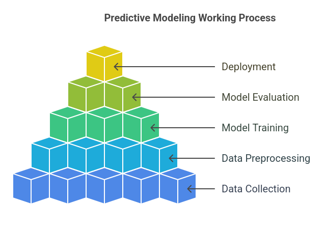
Step 1: Data Collection

Data is the foundation of predictive modeling. The quality, quantity, and relevance of the data significantly impact the accuracy of predictions.

Sources of Data:

• Structured Data: Databases (SQL, NoSQL), Spreadsheets, CRM systems
• Unstructured Data: Text documents, Images, Videos, Social Media
• Streaming Data: IoT sensors, Server logs, Web traffic
• Third-party Data: APIs, Government reports, Open datasets

Also Read: Difference Between Structured and Unstructured Data

Challenges in Data Collection:

• Data Inconsistency – Different sources may provide conflicting data.
• Data Gaps – Missing values in historical records.
• Data Privacy and Security – Regulatory compliance like GDPR and HIPAA.

Example: A retail company collects customer transaction history, website interactions, and social media engagement to predict future purchase behavior.

Step 2: Data Preprocessing & Feature Engineering

Raw data is often noisy, incomplete, or inconsistent. Preprocessing ensures data quality and prepares it for model training.

Key Steps in Data Preprocessing:

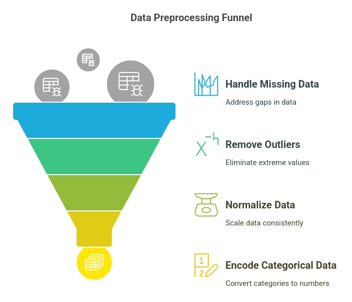
• Handling Missing Data:
  • Imputation (mean, median, mode)
  • Dropping rows/columns if missing data is excessive

• Removing Outliers:
  • Using Z-score, IQR (Interquartile Range), or clustering methods

• Data Normalization & Standardization:
  • Min-Max Scaling: Scales data between 0 and 1
  • Z-score Normalization: Standardizes data by subtracting the mean and dividing by the standard deviation

• Encoding Categorical Variables:
  • One-Hot Encoding: Converts categorical values into binary columns
  • Label Encoding: Assigns numerical values to categorical labels

Feature Engineering:

Feature engineering improves model performance by creating new relevant features from existing data.

• Combining Features: E.g., “Total Spend per Month” = “Number of Transactions” × “Average Spend”
• Extracting Time-based Features: E.g., Day of the week, Holiday, Seasonality in time-series data
• Text Processing: Tokenization, Lemmatization, and Sentiment Analysis for text data

Example: In fraud detection, new features like “Number of transactions per minute” can help identify suspicious activity.

Step 3: Model Selection & Training

Once the data is clean and transformed, the next step is selecting an appropriate model. The choice depends on the problem type (classification, regression, clustering, or time-series forecasting).

Types of Predictive Models:

1. Regression Models (Predicting Continuous Values):
   • Linear Regression (e.g., predicting house prices)
   • Logistic Regression (e.g., predicting the probability of customer churn)

2. Classification Models (Categorizing Data):
   • Decision Trees, Random Forest (e.g., spam detection)
   • Naïve Bayes (e.g., sentiment analysis)

3. Clustering Models (Grouping Similar Data Points):
   • K-Means Clustering (e.g., customer segmentation)

4. Time-Series Models (Forecasting Future Trends):
   • ARIMA, LSTMs (e.g., stock market predictions)

Model Training Process:

• Splitting Data:
  • Training Set (70-80%) – Used to train the model
  • Validation Set (10-15%) – Used to fine-tune hyperparameters
  • Test Set (10-15%) – Used to evaluate final model performance

• Hyperparameter Tuning: Adjusting model parameters to optimize performance using techniques like Grid Search and Random Search.

• Optimization Algorithms:
  • Gradient Descent (used in deep learning models)
  • Adam Optimizer (adaptive learning rate optimization)

Example: A healthcare provider trains a deep learning model using patient medical records to predict disease risks.

Step 4: Model Evaluation & Validation

Once trained, the model needs to be evaluated for accuracy, generalizability, and reliability.

Common Evaluation Metrics:

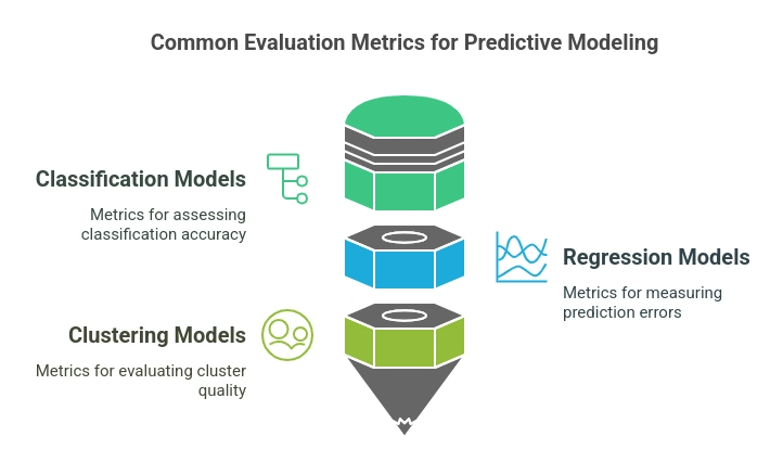
1. For Classification Models:
   • Accuracy – Percentage of correct predictions
   • Precision & Recall – Measures the relevance of positive predictions
   • F1-Score – Balances precision and recall
   • ROC-AUC Score – Evaluates classification performance across all probability thresholds

2. For Regression Models:
   • Mean Absolute Error (MAE) – Average absolute error of predictions
   • Mean Squared Error (MSE) – Penalizes larger errors
   • R² Score – Measures how well predictions fit actual data

3. For Clustering Models:
   • Silhouette Score – Evaluates how well clusters are formed
   • Elbow Method – Determines the optimal number of clusters

Cross-Validation Techniques:

• K-Fold Cross Validation: Splits data into multiple subsets to avoid overfitting.
• Leave-One-Out Cross Validation (LOOCV): Tests model on one observation at a time.

Example: A financial institution evaluates its credit risk prediction model using ROC-AUC scores before deployment.

Step 5: Deployment & Continuous Improvement

Once a model is validated, it is deployed into a real-world application. However, models need continuous monitoring and updates to maintain accuracy over time.

Deployment Strategies:

• Batch Processing: Predictions are generated at scheduled intervals (e.g., daily customer churn reports).
• Real-time Prediction: Models provide instant predictions via APIs (e.g., fraud detection during transactions).

Model Monitoring & Maintenance:

• Concept Drift: When the relationship between input and output changes over time, leading to model degradation.
• Performance Tracking: Automated monitoring dashboards track key performance metrics.
• Retraining Models: Updating models periodically with fresh data to maintain accuracy.

Continuous Learning:

• Online Learning Models: Some ML models learn from new data in real time without retraining from scratch.
• A/B Testing: Running multiple models in parallel to determine the best-performing one.
• Example: A ride-sharing app continuously updates its demand prediction model as user behavior changes.

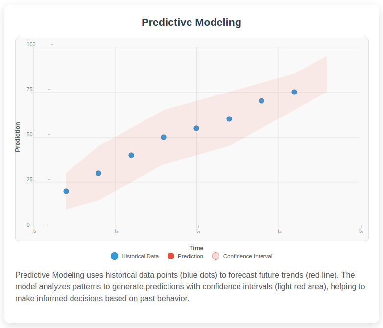
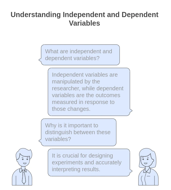
Difference Between Independent And Dependent Variable

Feature	Independent Variable	Dependent Variable
Definition	Variables that are manipulated to observe their effect.	Variables that are measured or predicted, depending on the independent variable.
Role in an Experiment	Acts as inputs or predictors.	Serves as outputs or responses.
Example	In a study, hours spent studying.	The resulting test scores, dependent on study hours.
Nature	Can be continuous (age, height) or categorical (sex, treatment type).	Can also be continuous (test scores, weight) or categorical (yes/no outcomes).
Manipulation	Can be controlled or changed by researchers.	Observed in response to changes in the independent variable.
Graphical Representation	Often represented on the x-axis.	Usually represented on the y-axis.
Purpose in Analysis	Used to determine its effect on the dependent variable.	To understand its change due to the independent variable.
Example in Regression	Used to predict the dependent variable.	The target being predicted based on the independent variable.
Confidence Intervals	Not usually tested for significance.	Associated with statistical tests to measure prediction confidence.
Direction of Influence	Hypothesized to influence dependent variables.	Affected by independent variables.

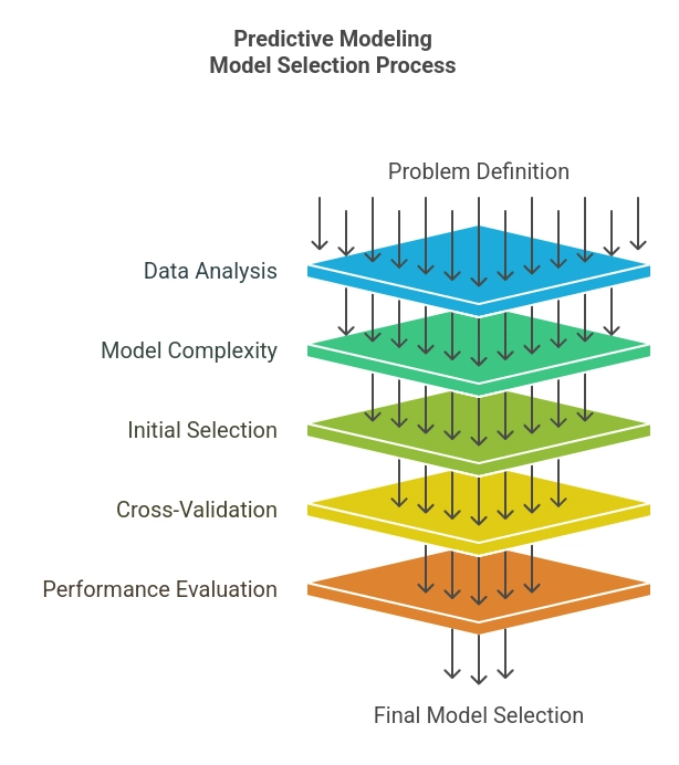
How To Select The Right Model?

1. Understand the Problem

• Define the Objective: What are you trying to predict? Is it a classification or regression problem? Understanding the goal helps narrow down model choices.

• Determine Success Metrics: Define how you will measure the success of the model (e.g., accuracy, precision, recall, F1 score, ROC-AUC for classification; RMSE, MAE for regression).

2. Analyze the Data

• Exploratory Data Analysis (EDA): Conduct EDA to understand the structure, distribution, and relationships within the data. Look for outliers, missing values, and patterns.

• Feature Types: Identify the types of features (numerical, categorical, ordinal) and their distributions, which will influence model suitability.

• Size of the Dataset: Consider the size of your dataset. Some models (like neural networks) require large data sets, while simpler methods (like linear regression) may be effective with smaller datasets.

3. Consider Model Complexity

• Bias-Variance Tradeoff: Simple models often have high bias and low variance, while complex models may have low bias but high variance. Balance is crucial—choose a model that is complex enough to capture the underlying patterns but simple enough to generalize well on unseen data.

• Interpretable vs. Black-Box Models: If interpretability is important (for example, in healthcare or finance), you might prefer simpler models (like logistic regression or decision trees), whereas, in other cases, you might prioritize accuracy.

4. Initial Model Selection

• Baseline Model: Start with a simple model as a baseline (such as linear regression or logistic regression) to establish a performance benchmark.

• Test Various Models: Evaluate a diverse set of models relevant to the problem, such as decision trees, random forests, support vector machines (SVM), gradient boosting machines (GBM), or neural networks.

5. Cross-Validation

• K-Fold Cross-Validation: Use techniques like k-fold cross-validation to get a more reliable estimate of model performance. This helps to understand how the model performs on different subsets of data and mitigates overfitting.

• Hyperparameter Tuning: Optimize the chosen models using techniques like Grid Search or Random Search to find the best parameters.

6. Evaluate Model Performance

• Use Multiple Metrics: Don’t rely on a single metric to assess model performance. For classification, consider precision, recall, F1 score, ROC-AUC; for regression, consider RMSE, MAE, and R-squared.

• Analyze Errors: Look at where and why the model is making errors. This can provide insights into whether a different model might suit the data better.

7. Feature Engineering

• Feature Importance: Assess and select key features that contribute meaningfully to the predictions. Some models, like decision trees and random forests, provide built-in feature importance metrics.

• Transformations: Explore feature engineering techniques, such as normalization, scaling, encoding categorical variables, or creating new features based on domain knowledge.

8. Final Model Selection

• Trade-offs: Consider the trade-offs among various models in terms of accuracy, interpretability, training time, inference time, and computational resources.

• Business Context: Choose a model that not only performs well statistically but also aligns with the organizational context, deployment strategy, and operational constraints.

9. Iterate and Improve

• Feedback Loop: Monitor the model’s performance over time. Gather new data and feedback to continually refine and update the model.

• Experimentation: Don’t hesitate to experiment with different models periodically to test if improvements can be made, especially as new data becomes available.

Selecting the right predictive model is an iterative process that relies on a solid understanding of the problem, data characteristics, and the models themselves.

By following these structured steps, you can make an informed decision that ultimately leads to more reliable predictions and better outcomes for your specific application.

Conclusion 

Predictive modeling is transforming industries with data-driven decision-making, risk estimation, and forecasting the future. To become proficient in predictive analytics, you need a strong grasp of machine learning, data preprocessing, and model evaluation.

If you wish to develop expertise in data science and analytics, the MIT Data Science and Machine Learning Course offers hands-on training, live projects, and industry-specific insights to make you proficient in this highly-demanding sector.