
Imagine training a model on raw data without cleaning, transforming, or optimizing it.
The results?
Poor predictions, wasted resources, and suboptimal performance. Feature engineering is the art of extracting the most relevant insights from data, ensuring that machine learning models work efficiently.
Whether you're dealing with structured data, text, or images, mastering feature engineering can be a game-changer. This guide covers the most effective techniques and best practices to help you build high-performance models.
What is Feature Engineering?
Feature engineering is the art of converting raw data into useful input variables (features) that improve the performance of machine learning models. It helps in choosing the most useful features to enhance a model's capacity to learn patterns & make good predictions.
Feature engineering encompasses methods like feature scaling, encoding categorical variables, feature selection, and building interaction terms.
Why is Feature Engineering Important?
Feature engineering is one of the most critical steps in machine learning. Even the most advanced algorithms can fail if they are trained on poorly designed features. Here’s why it matters:
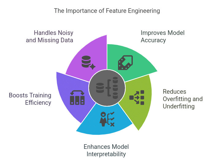
1. Improves Model Accuracy
A well-engineered feature set allows a model to capture patterns more effectively, leading to higher accuracy. For example, converting a date column into “day of the week” or “holiday vs. non-holiday” can improve sales forecasting models.
2. Reduces Overfitting and Underfitting
By removing irrelevant or highly correlated features, feature engineering prevents the model from memorizing noise (overfitting) and ensures it generalizes well on unseen data.
3. Enhances Model Interpretability
Features that align with domain knowledge make the model's decisions more explainable. For instance, in fraud detection, a feature like "number of transactions per hour" is more informative than raw timestamps.
4. Boosts Training Efficiency
Reducing the number of unnecessary features decreases computational complexity, making training faster and more efficient.
5. Handles Noisy and Missing Data
Raw data is often incomplete or contains outliers. Feature engineering helps clean and structure this data, ensuring better learning outcomes.
Also Read: What is Predictive Modeling?
Key Methods of Feature Engineering
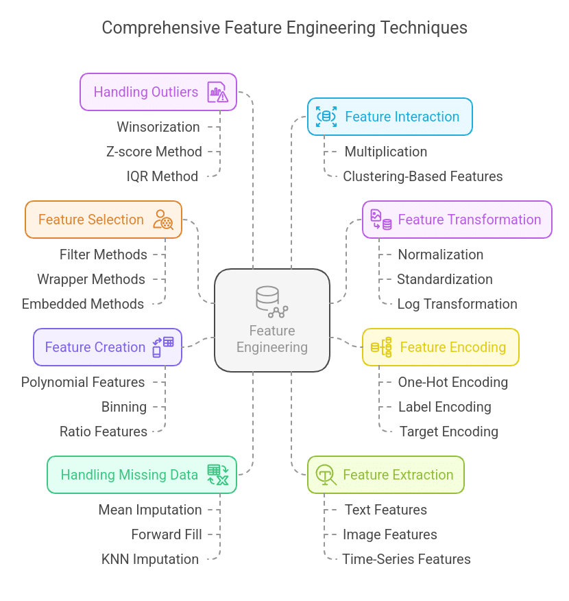
1. Feature Selection
Selecting the most relevant features while eliminating redundant, irrelevant, or highly correlated variables helps improve model efficiency and accuracy.
Techniques:
- Filter Methods: Uses statistical techniques like correlation, variance threshold, or mutual information to select important features.
- Wrapper Methods: Uses iterative techniques like Recursive Feature Elimination (RFE) and stepwise selection.
- Embedded Methods: Feature selection is built into the algorithm, such as Lasso Regression (L1 regularization) or decision tree-based models.
Example: Removing highly correlated features like "Total Sales" and "Average Monthly Sales" if one can be derived from the other.
2. Feature Transformation
Transforms raw data to improve model learning by making it more interpretable or reducing skewness.
Techniques:
- Normalization (Min-Max Scaling): Rescales values between 0 and 1. Useful for distance-based models like k-NN.
- Standardization (Z-score Scaling): Transforms data to have a mean of 0 and standard deviation of 1. Works well for gradient-based models like logistic regression.
- Log Transformation: Converts skewed data into a normal distribution.
- Power Transformation (Box-Cox, Yeo-Johnson): Used to stabilize variance and make data more normal-like.
Example: Scaling customer income before using it in a model to prevent high-value dominance.
3. Feature Encoding
Categorical features must be converted into numerical values for machine learning models to process.
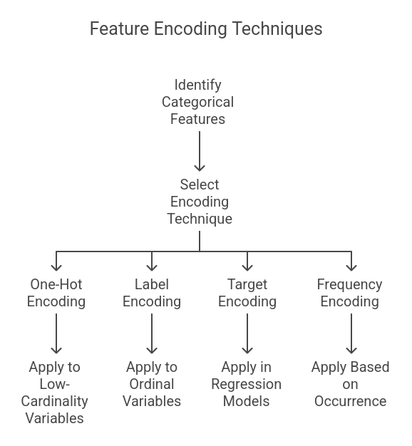
Techniques:
- One-Hot Encoding (OHE): Creates binary columns for each category (suitable for low-cardinality categorical variables).
- Label Encoding: Assigns numerical values to categories (useful for ordinal categories like "low," "medium," "high").
- Target Encoding: Replaces categories with the mean target value (commonly used in regression models).
- Frequency Encoding: Converts categories into their occurrence frequency in the dataset.
Example: Converting "City" into multiple binary columns using one-hot encoding:
| City | New York | San Francisco | Chicago |
| NY | 1 | 0 | 0 |
| SF | 0 | 1 | 0 |
4. Feature Creation (Derived Features)
Feature creation involves constructing new features from existing ones to provide additional insights and improve model performance. Well-crafted features can capture hidden relationships in data, making patterns more evident to machine learning models.
Techniques:
- Polynomial Features: Useful for models that need to capture non-linear relationships between variables.
- Example: If a model struggles with a linear relationship, adding polynomial terms like x², x³, or interaction terms (x1 * x2) can improve performance.
- Use Case: Predicting house prices based on features like square footage and number of rooms. Instead of just using square footage, a model could benefit from an interaction term like square_footage * number_of_rooms.
- Binning (Discretization): Converts continuous variables into categorical bins to simplify the relationship.
- Example: Instead of using raw age values (22, 34, 45), we can group them into bins:
- Young (18-30)
- Middle-aged (31-50)
- Senior (51+)
- Use Case: Credit risk modeling, where different age groups have different risk levels.
- Example: Instead of using raw age values (22, 34, 45), we can group them into bins:
- Ratio Features: Creating ratios between two related numerical values to normalize the impact of scale.
- Example: Instead of using income and loan amount separately, use Income-to-Loan Ratio = Income / Loan Amount to standardize comparisons across different income levels.
- Use Case: Loan default prediction, where individuals with a higher debt-to-income ratio are more likely to default.
- Time-based Features: Extracts meaningful insights from timestamps, such as:
- Hour of the day (helps in traffic analysis)
- Day of the week (useful for sales forecasting)
- Season (important for retail and tourism industries)
- Use Case: Predicting e-commerce sales by analyzing trends based on weekdays vs. weekends.
Example:
| Timestamp | Hour | Day of Week | Month | Season |
| 2024-02-15 14:30 | 14 | Thursday | 2 | Winter |
| 2024-06-10 08:15 | 8 | Monday | 6 | Summer |
5. Handling Missing Data
Missing data is common in real-world datasets and can negatively impact model performance if not handled properly. Instead of simply dropping missing values, feature engineering techniques help retain valuable information while minimizing bias.
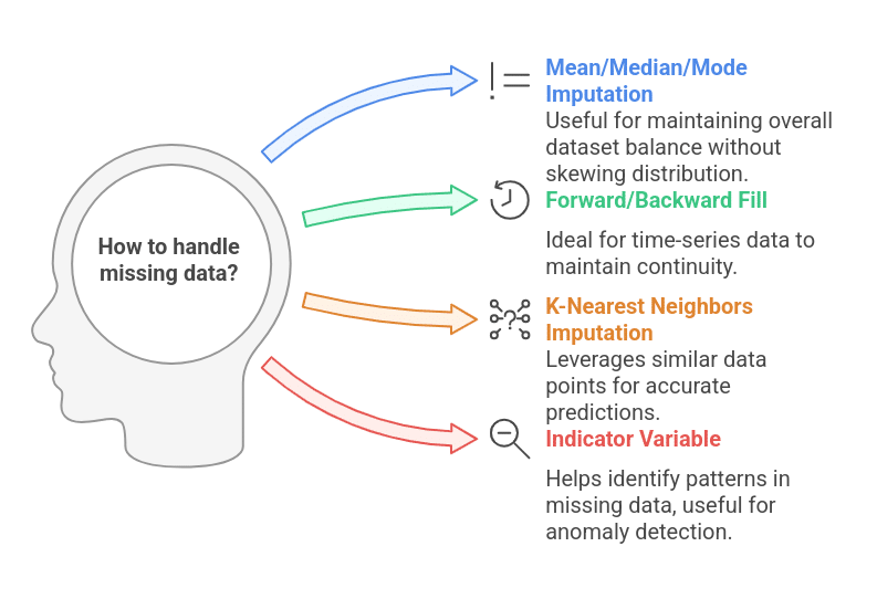
Techniques:
- Mean/Median/Mode Imputation:
- Fills missing values with the mean (for numerical data) or mode (for categorical data).
- Example: Filling missing salary values with the median salary of the dataset to prevent skewing the distribution.
- Forward or Backward Fill (Time-Series Data):
- Forward fill: Uses the last known value to fill missing entries.
- Backward fill: Uses the next known value to fill missing entries.
- Use Case: Stock market data where missing prices can be filled with the previous day's prices.
- K-Nearest Neighbors (KNN) Imputation:
- Uses similar data points to estimate missing values.
- Example: If a person’s income is missing, KNN can predict it based on people with similar job roles, education levels, and locations.
- Indicator Variable for Missingness:
- Creates a binary column (1 = Missing, 0 = Present) to retain missing data patterns.
- Use Case: Detecting fraudulent transactions where missing values themselves may indicate suspicious activity.
Example:
| Customer ID | Age | Salary | Salary Missing Indicator |
| 101 | 35 | 50,000 | 0 |
| 102 | 42 | NaN | 1 |
| 103 | 29 | 40,000 | 0 |
6. Feature Extraction
Feature extraction involves deriving new, meaningful representations from complex data formats like text, images, and time-series. This is especially useful in high-dimensional datasets.
Techniques:
- Text Features: Converts textual data into numerical form for machine learning models.
- Bag of Words (BoW): Represents text as word frequencies in a matrix.
- TF-IDF (Term Frequency-Inverse Document Frequency): Gives importance to words based on their frequency in a document vs. overall dataset.
- Word Embeddings (Word2Vec, GloVe, BERT): Captures semantic meaning of words.
- Use Case: Sentiment analysis of customer reviews.
- Image Features: Extract essential patterns from images.
- Edge Detection: Identifies object boundaries in images (useful in medical imaging).
- Histogram of Oriented Gradients (HOG): Used in object detection.
- CNN-based Feature Extraction: Uses deep learning models like ResNet and VGG for automatic feature learning.
- Use Case: Facial recognition, self-driving car object detection.
- Time-Series Features: Extract meaningful trends and seasonality from time-series data.
- Rolling Averages: Smooth out short-term fluctuations.
- Seasonal Decomposition: Separates trend, seasonality, and residual components.
- Autoregressive Features: Uses past values as inputs for predictive models.
- Use Case: Forecasting electricity demand based on historical consumption patterns.
- Dimensionality Reduction (PCA, t-SNE, UMAP):
- PCA (Principal Component Analysis) reduces high-dimensional data while preserving variance.
- t-SNE and UMAP are useful for visualizing clusters in large datasets.
- Use Case: Reducing thousands of customer behavior variables into a few principal components for clustering.
Example:
For text analysis, TF-IDF converts raw sentences into numerical form:
| Sentence | "AI is transforming healthcare" | "AI is advancing research" |
| AI | 0.4 | 0.3 |
| transforming | 0.6 | 0.0 |
| research | 0.0 | 0.7 |
7. Handling Outliers
Outliers are extreme values that can distort a model’s predictions. Identifying and handling them properly prevents skewed results.
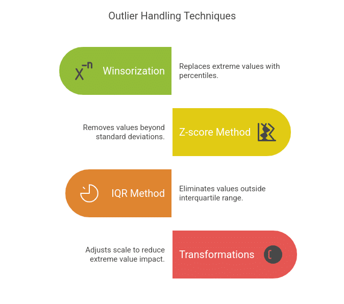
Techniques:
- Winsorization: Replaces extreme values with a specified percentile (e.g., capping values at the 5th and 95th percentile).
- Z-score Method: Removes values that are more than a certain number of standard deviations from the mean (e.g., ±3σ).
- IQR (Interquartile Range) Method: Removes values beyond 1.5 times the interquartile range (Q1 and Q3).
- Transformations (Log, Square Root): Reduces the impact of extreme values by adjusting scale.
Example:
Detecting outliers in a salary dataset using IQR:
| Employee | Salary | Outlier (IQR Method) |
| A | 50,000 | No |
| B | 52,000 | No |
| C | 200,000 | Yes |
8. Feature Interaction
Feature interaction helps capture relationships between variables that aren’t obvious in their raw form.
Techniques:
- Multiplication or Division of Features:
- Example: Instead of using "Weight" and "Height" separately, create BMI = Weight / Height².
- Polynomial Features:
- Example: Adding squared or cubic terms for better non-linear modelling.
- Clustering-Based Features:
- Assign cluster labels using k-means, which can be used as categorical inputs.
Example:
Creating an "Engagement Score" for a user based on:
Engagement Score = (Logins * Time Spent) / (1 + Bounce Rate).
By leveraging these feature engineering techniques, you can transform raw data into powerful predictive inputs, ultimately improving model accuracy, efficiency, and interoperability.
Comparison: Good vs. Bad Feature Engineering
Data Preprocessing
Good Feature Engineering
Handles missing values, removes outliers, and applies proper scaling.
Bad Feature Engineering
Ignores missing values, includes outliers, and fails to standardize.
Feature Selection
Good Feature Engineering
Uses correlation analysis, importance scores, and domain expertise to pick features.
Bad Feature Engineering
Uses all features, even if some are redundant or irrelevant.
Feature Transformation
Good Feature Engineering
Normalizes, scales, and applies log transformations when necessary.
Bad Feature Engineering
Uses raw data without processing, leading to inconsistent model behavior.
Encoding Categorical Data
Good Feature Engineering
Uses proper encoding techniques like one-hot, target, or frequency encoding.
Bad Feature Engineering
Assigns arbitrary numeric values to categories, misleading the model.
Feature Creation
Good Feature Engineering
Introduces meaningful new features (e.g., ratios, interactions, polynomial terms).
Bad Feature Engineering
Adds random variables or duplicates existing features.
Handling Time-based Data
Good Feature Engineering
Extracts useful patterns (e.g., day of the week, trend indicators).
Bad Feature Engineering
Leaves timestamps in raw format, making patterns harder to learn.
Model Performance
Good Feature Engineering
Higher accuracy, generalizes well on new data, interpretable results.
Bad Feature Engineering
Poor accuracy, overfits training data, fails in real-world scenarios.
How Does Good and Bad Feature Engineering Affect Model Performance?
Example 1: Predicting House Prices
- Good Feature Engineering: Instead of using the raw "Year Built" column, create a new feature: "House Age" (Current Year - Year Built). This provides a clearer relationship with price.
- Bad Feature Engineering: Keeping the "Year Built" column as-is, forcing the model to learn complex patterns instead of focusing on a straightforward numerical relationship.
Example 2: Credit Card Fraud Detection
- Good Feature Engineering: Creating a new feature "Number of Transactions in the Last Hour" helps identify suspicious activity.
- Bad Feature Engineering: Using raw timestamps without any transformation, making it difficult for the model to detect time-based anomalies.
Example 3: Customer Churn Prediction
- Good Feature Engineering: Combining customer interaction data into a "Monthly Activity Score" (e.g., logins, purchases, support queries).
- Bad Feature Engineering: Using each interaction type separately, making the dataset unnecessarily complex and harder for the model to interpret.
Best Practices in Feature Engineering
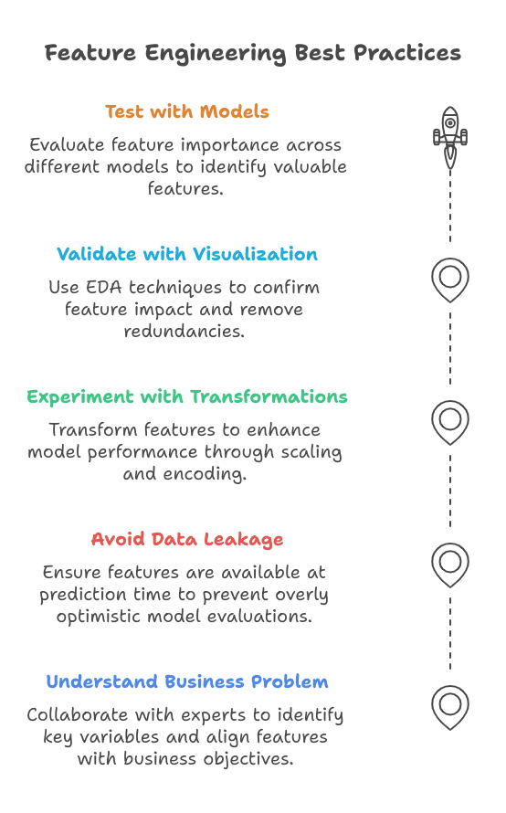
1. Understanding the Business Problem Before Selecting Features
Before applying feature engineering techniques, it’s crucial to understand the specific problem the model aims to solve. Selecting features without considering the domain context can lead to irrelevant or misleading inputs, reducing model effectiveness.
Best Practices:
- Collaborate with domain experts to identify key variables.
- Analyze historical trends and real-world constraints.
- Ensure selected features align with business objectives.
Example:
For a loan default prediction model, features like credit score, income stability, and past loan repayment behavior are more valuable than generic features like ZIP code.
2. Avoiding Data Leakage Through Careful Feature Selection
Data leakage occurs when information from the training set is inadvertently included in the test set, leading to overly optimistic performance that does not generalize well to real-world scenarios.
Best Practices:
- Exclude features that wouldn’t be available at the time of prediction.
- Avoid using future information in training data.
- Be cautious with derived features based on target variables.
Example of Data Leakage:
Using “total purchases in the next 3 months” as a feature to predict customer churn. Since this information wouldn’t be available at the prediction time, it would lead to incorrect model evaluation.
Fix: Use past purchase behavior (e.g., "number of purchases in the last 6 months") instead.
3. Experimenting with Different Transformations and Encodings
Transforming features into more suitable formats can significantly enhance model performance. This includes scaling numerical variables, encoding categorical variables, and applying mathematical transformations.
Best Practices:
- Scaling numerical variables (Min-Max Scaling, Standardization) to ensure consistency.
- Encoding categorical variables (One-Hot, Label Encoding, Target Encoding) based on data distribution.
- Applying transformations (Log, Square Root, Power Transform) to normalize skewed data.
Example:
For a dataset with highly skewed income data:
- Raw Income Data: [10,000, 20,000, 50,000, 1,000,000] (skewed distribution)
- Log Transformation: [4, 4.3, 4.7, 6] (reduces skewness, improving model performance).
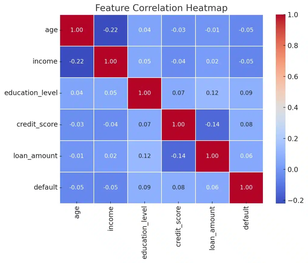
4. Validating Engineered Features Using Visualization and Correlation Analysis
Before finalizing features, it’s essential to validate their impact using exploratory data analysis (EDA) techniques.
Best Practices:
- Use histograms and box plots to check feature distributions.
- Use scatter plots and correlation heatmaps to identify relationships between variables.
- Remove highly correlated features to prevent multicollinearity.
Example:
In a sales prediction model, if "marketing spend" and "ad budget" have a correlation > 0.9, keeping both could introduce redundancy. Instead, use one or create a derived feature like "marketing efficiency = revenue/ad spend".
5. Testing Features with Different Models to Evaluate Impact
Feature importance varies across different algorithms. A feature that improves performance in one model might not be useful in another.
Best Practices:
- Train multiple models (Linear Regression, Decision Trees, Neural Networks) and compare feature importance.
- Use Permutation Importance or SHAP values to understand each feature’s contribution.
- Perform Ablation Studies (removing one feature at a time) to measure performance impact.
Example:
In a customer churn model:
- Decision trees might prioritize customer complaints and contract types.
- Logistic regression might find tenure and monthly bill amounts more significant.
By testing different models, you can identify the most valuable features.
Tools for Feature Engineering
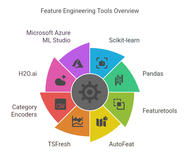
1. Python Libraries for Feature Engineering
Python is the go-to language for feature engineering due to its robust libraries:
- Pandas – For data manipulation, feature extraction, and handling missing values.
- NumPy – For mathematical operations and transformations on numerical data.
- Scikit-learn – For preprocessing techniques like scaling, encoding, and feature selection.
- Feature-engine – A specialized library with transformers for handling outliers, imputation, and categorical encoding.
- Scipy – Useful for statistical transformations, like polynomial feature generation and power transformations.
Also Read: List of Python Libraries for Data Science and Analysis
2. Automated Feature Engineering Tools
- Featuretools – Automates the creation of new features using deep feature synthesis (DFS).
- tsfresh – Extracts meaningful time-series features like trend, seasonality, and entropy.
- AutoFeat – Automates feature extraction and selection using AI-driven techniques.
- H2O.ai AutoML – Performs automatic feature transformation and selection.
3. Big Data Tools for Feature Engineering
- Spark MLlib (Apache Spark) – Handles large-scale data transformations and feature extraction in distributed environments.
- Dask – Parallel processing for scaling feature engineering on large datasets.
- Feast (Feature Store by Tecton) – Manages and serves features efficiently for machine learning models in production.
4. Feature Selection and Importance Tools
- SHAP (Shapley Additive Explanations) – Measures feature importance and impact on predictions.
- LIME (Local Interpretable Model-agnostic Explanations) – Helps interpret individual predictions and assess feature relevance.
- Boruta – A wrapper method for selecting the most important features using a random forest algorithm.
5. Visualization Tools for Feature Engineering
- Matplotlib & Seaborn – For exploring feature distributions, correlations, and trends.
- Plotly – For interactive feature analysis and pattern detection.
- Yellowbrick – Provides visual diagnostics for feature selection and model performance.
Conclusion
Mastering feature engineering is essential for building high-performance machine learning models, and the right tools can significantly streamline the process.
Leveraging these tools, from data preprocessing with Pandas and Scikit-learn to automated feature extraction with Featuretools and SHAP for interpretability, can enhance model accuracy and efficiency.
To gain hands-on expertise in feature engineering and machine learning, take this free feature engineering course and elevate your career today!
Enroll in our MIT Data Science and Machine Learning Course to gain complete expertise in such data science and machine learning topics.


