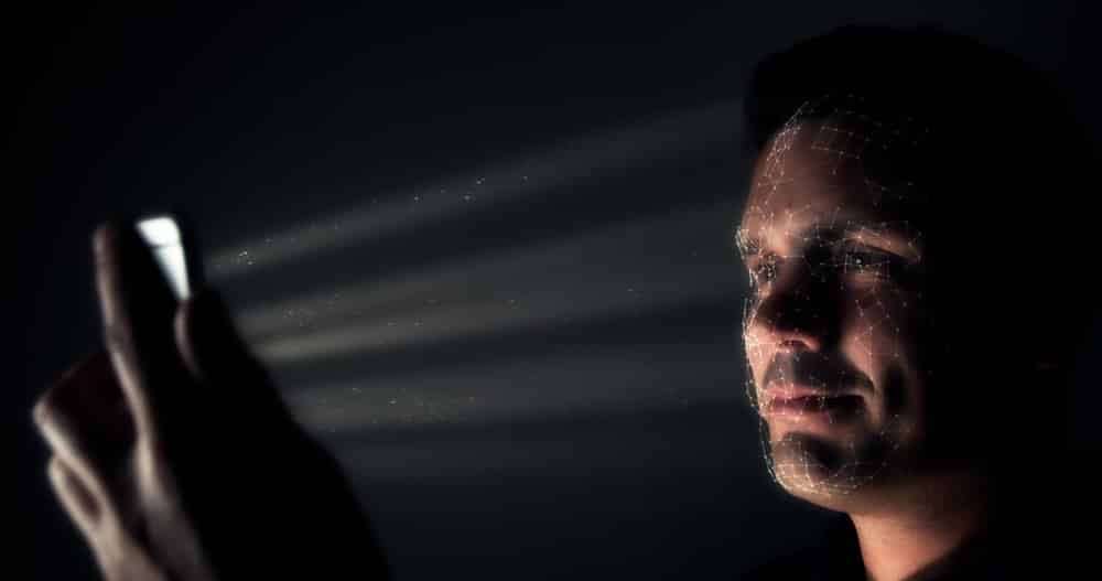
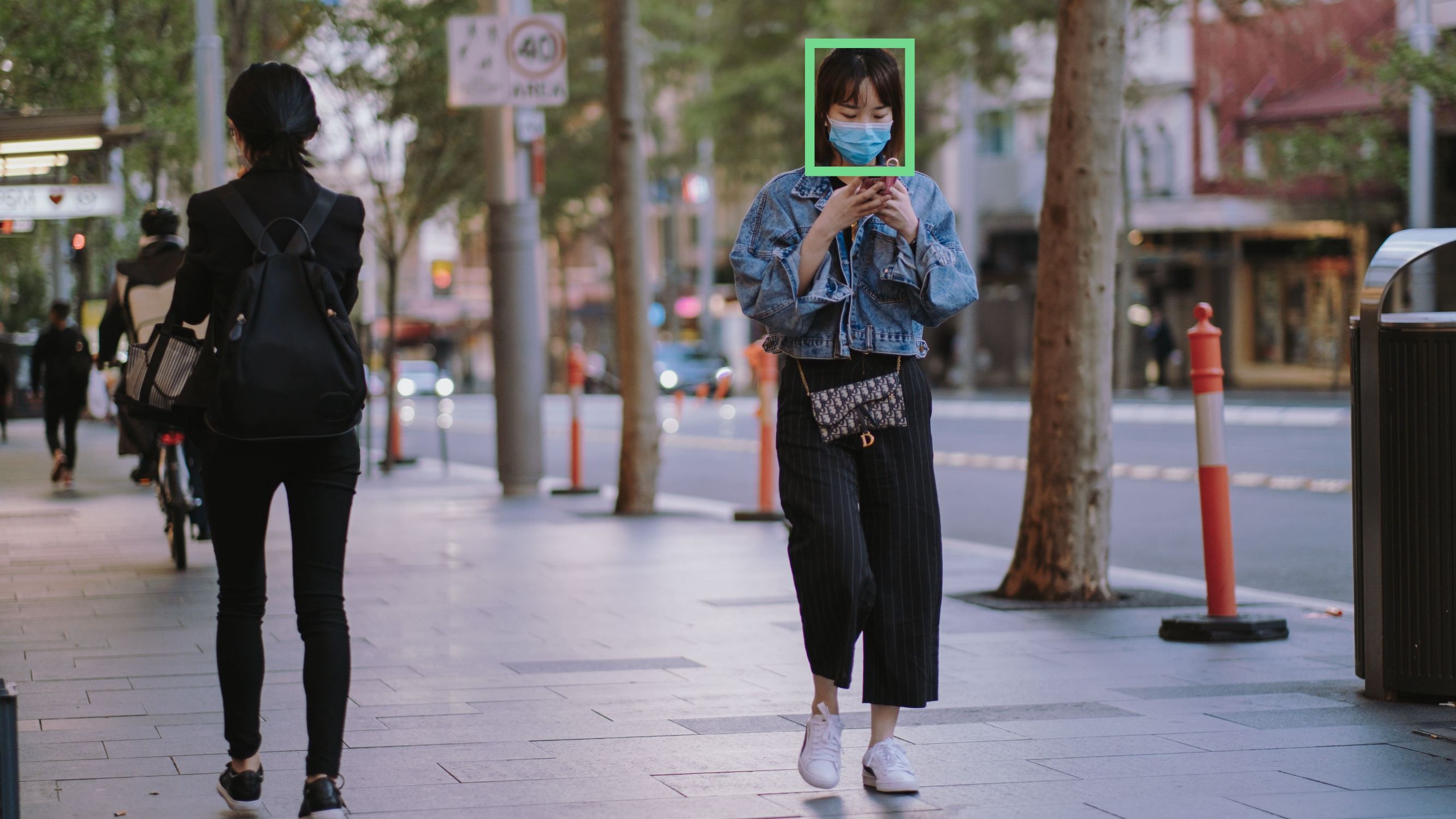
How to Detect Face Recognition using Viola Jones Algorithm

In the realm of computer vision, face detection stands as a fundamental and captivating task. Detecting and locating faces within images or video streams forms the cornerstone of numerous applications, from facial recognition systems to digital image processing. Among the many algorithms developed to tackle this challenge, the Viola-Jones algorithm has emerged as a groundbreaking approach renowned for its speed and accuracy.

The Viola-Jones algorithm, pioneered by Paul Viola and Michael Jones in 2001, revolutionized the field of face detection. Its efficient and robust methodology opened doors to a wide range of applications that rely on accurately identifying and analyzing human faces. By harnessing the power of Haar-like features, integral images, machine learning, and cascades of classifiers, the Viola-Jones algorithm showcases the synergy between computer science and image processing.

In this blog, we will delve into the intricacies of the Viola-Jones algorithm, unraveling its underlying mechanisms and exploring its applications. From its training process to its implementation in real-world scenarios, we will unlock the power of face detection and witness firsthand the transformative capabilities of the Viola-Jones algorithm.

What is face detection?
What is Viola Jones algorithm?
Using a Viola Jones Classifier to detect faces in a live webcam feed

What is face detection?

Object detection is one of the computer technologies that is connected to image processing and computer vision. It is concerned with detecting instances of an object such as human faces, buildings, trees, cars, etc. The primary aim of face detection algorithms is to determine whether there is any face in an image or not.

In recent years, we have seen significant advancement of technologies that can detect and recognise faces. Our mobile cameras are often equipped with such technology where we can see a box around the faces. Although there are quite advanced face detection algorithms, especially with the introduction of deep learning, the introduction of viola jones algorithm in 2001 was a breakthrough in this field. Now let us explore the viola jones algorithm in detail.

What is Viola Jones algorithm?

Viola Jones algorithm is named after two computer vision researchers who proposed the method in 2001, Paul Viola and Michael Jones in their paper, “Rapid Object Detection using a Boosted Cascade of Simple Features”. Despite being an outdated framework, Viola-Jones is quite powerful, and its application has proven to be exceptionally notable in real-time face detection. This algorithm is painfully slow to train but can detect faces in real-time with impressive speed.

Given an image(this algorithm works on grayscale image), the algorithm looks at many smaller subregions and tries to find a face by looking for specific features in each subregion. It needs to check many different positions and scales because an image can contain many faces of various sizes. Viola and Jones used Haar-like features to detect faces in this algorithm.

The Viola Jones algorithm has four main steps, which we shall discuss in the sections to follow:

Selecting Haar-like features
Creating an integral image
Running AdaBoost training
Creating classifier cascades

What are Haar-Like Features?

In the 19th century a Hungarian mathematician, Alfred Haar gave the concepts of Haar wavelets, which are a sequence of rescaled “square-shaped” functions which together form a wavelet family or basis. Voila and Jones adapted the idea of using Haar wavelets and developed the so-called Haar-like features.

Haar-like features are digital image features used in object recognition. All human faces share some universal properties of the human face like the eyes region is darker than its neighbour pixels, and the nose region is brighter than the eye region.

A simple way to find out which region is lighter or darker is to sum up the pixel values of both regions and compare them. The sum of pixel values in the darker region will be smaller than the sum of pixels in the lighter region. If one side is lighter than the other, it may be an edge of an eyebrow or sometimes the middle portion may be shinier than the surrounding boxes, which can be interpreted as a nose This can be accomplished using Haar-like features and with the help of them, we can interpret the different parts of a face.

There are 3 types of Haar-like features that Viola and Jones identified in their research:

Edge features
Line-features
Four-sided features

Edge features and Line features are useful for detecting edges and lines respectively. The four-sided features are used for finding diagonal features.

The value of the feature is calculated as a single number: the sum of pixel values in the black area minus the sum of pixel values in the white area. The value is zero for a plain surface in which all the pixels have the same value, and thus, provide no useful information.

Since our faces are of complex shapes with darker and brighter spots, a Haar-like feature gives you a large number when the areas in the black and white rectangles are very different. Using this value, we get a piece of valid information out of the image.

To be useful, a Haar-like feature needs to give you a large number, meaning that the areas in the black and white rectangles are very different. There are known features that perform very well to detect human faces:

For example, when we apply this specific haar-like feature to the bridge of the nose, we get a good response. Similarly, we combine many of these features to understand if an image region contains a human face.

What are Integral Images?

In the previous section, we have seen that to calculate a value for each feature, we need to perform computations on all the pixels inside that particular feature. In reality, these calculations can be very intensive since the number of pixels would be much greater when we are dealing with a large feature.

The integral image plays its part in allowing us to perform these intensive calculations quickly so we can understand whether a feature of several features fit the criteria.

An integral image (also known as a summed-area table) is the name of both a data structure and an algorithm used to obtain this data structure. It is used as a quick and efficient way to calculate the sum of pixel values in an image or rectangular part of an image.

How is AdaBoost used in viola jones algorithm?

Next, we use a Machine Learning algorithm known as AdaBoost. But why do we even want an algorithm?

The number of features that are present in the 24×24 detector window is nearly 160,000, but only a few of these features are important to identify a face. So we use the AdaBoost algorithm to identify the best features in the 160,000 features.

In the Viola-Jones algorithm, each Haar-like feature represents a weak learner. To decide the type and size of a feature that goes into the final classifier, AdaBoost checks the performance of all classifiers that you supply to it.

To calculate the performance of a classifier, you evaluate it on all subregions of all the images used for training. Some subregions will produce a strong response in the classifier. Those will be classified as positives, meaning the classifier thinks it contains a human face. Subregions that don’t provide a strong response don’t contain a human face, in the classifiers opinion. They will be classified as negatives.

The classifiers that performed well are given higher importance or weight. The final result is a strong classifier, also called a boosted classifier, that contains the best performing weak classifiers.

So when we’re training the AdaBoost to identify important features, we’re feeding it information in the form of training data and subsequently training it to learn from the information to predict. So ultimately, the algorithm is setting a minimum threshold to determine whether something can be classified as a useful feature or not.

What are Cascading Classifiers?

Maybe the AdaBoost will finally select the best features around say 2500, but it is still a time-consuming process to calculate these features for each region. We have a 24×24 window which we slide over the input image, and we need to find if any of those regions contain the face. The job of the cascade is to quickly discard non-faces, and avoid wasting precious time and computations. Thus, achieving the speed necessary for real-time face detection.

We set up a cascaded system in which we divide the process of identifying a face into multiple stages. In the first stage, we have a classifier which is made up of our best features, in other words, in the first stage, the subregion passes through the best features such as the feature which identifies the nose bridge or the one that identifies the eyes. In the next stages, we have all the remaining features.

When an image subregion enters the cascade, it is evaluated by the first stage. If that stage evaluates the subregion as positive, meaning that it thinks it’s a face, the output of the stage is maybe.

When a subregion gets a maybe, it is sent to the next stage of the cascade and the process continues as such till we reach the last stage.

If all classifiers approve the image, it is finally classified as a human face and is presented to the user as a detection.

Now how does it help us to increase our speed? Basically, If the first stage gives a negative evaluation, then the image is immediately discarded as not containing a human face. If it passes the first stage but fails the second stage, it is discarded as well. Basically, the image can get discarded at any stage of the classifier

Using a Viola-Jones Classifier to detect faces in a live webcam feed

In this section, we are going to implement the Viola-Jones algorithm using OpenCV and detect faces in our webcam feed in real-time. We will also use the same algorithm to detect the eyes of a person too. This is quite simple and all you need is to install OpenCV and Python on your PC. You can refer to this article to know about OpenCV and how to install it

In OpenCV, we have several trained Haar Cascade models which are saved as XML files. Instead of creating and training the model from scratch, we use this file. We are going to use “haarcascade_frontalface_alt2.xml” file in this project. Now let us start coding.

The first step is to find the path to the “haarcascade_frontalface_alt2.xml” and “haarcascade_eye_tree_eyeglasses.xml” files. We do this by using the os module of Python language.

import os
cascPathface = os.path.dirname(
    cv2.__file__) + "/data/haarcascade_frontalface_alt2.xml"
cascPatheyes = os.path.dirname(
    cv2.__file__) + "/data/haarcascade_eye_tree_eyeglasses.xml"

The next step is to load our classifier. We are using two classifiers, one for detecting the face and others for detection eyes. The path to the above XML file goes as an argument to CascadeClassifier() method of OpenCV.

faceCascade = cv2.CascadeClassifier(cascPath)
eyeCascade = cv2.CascadeClassifier(cascPatheyes)

After loading the classifier, let us open the webcam using this simple OpenCV one-liner code

video_capture = cv2.VideoCapture(0)

Next, we need to get the frames from the webcam stream, we do this using the read() function. We use the infinite loop to get all the frames until the time we want to close the stream.

while True:
    # Capture frame-by-frame
    ret, frame = video_capture.read()

The read() function returns:

The actual video frame read (one frame on each loop)
A return code

The return code tells us if we have run out of frames, which will happen if we are reading from a file. This doesn’t matter when reading from the webcam since we can record forever, so we will ignore it.

For this specific classifier to work, we need to convert the frame into greyscale.

gray = cv2.cvtColor(frame, cv2.COLOR_BGR2GRAY)

The faceCascade object has a method detectMultiScale(), which receives a frame(image) as an argument and runs the classifier cascade over the image. The term MultiScale indicates that the algorithm looks at subregions of the image in multiple scales, to detect faces of varying sizes.

faces = faceCascade.detectMultiScale(gray,
                                         scaleFactor=1.1,
                                         minNeighbors=5,
                                         minSize=(60, 60),
                                         flags=cv2.CASCADE_SCALE_IMAGE)

Let us go through these arguments of this function:

scaleFactor – Parameter specifying how much the image size is reduced at each image scale. By rescaling the input image, you can resize a larger face to a smaller one, making it detectable by the algorithm. 1.05 is a good possible value for this, which means you use a small step for resizing, i.e. reduce the size by 5%, you increase the chance of a matching size with the model for detection is found.
minNeighbors – Parameter specifying how many neighbours each candidate rectangle should have to retain it. This parameter will affect the quality of the detected faces. Higher value results in fewer detections but with higher quality. 3~6 is a good value for it.
flags –Mode of operation
minSize – Minimum possible object size. Objects smaller than that are ignored.

The variable faces now contain all the detections for the target image. Detections are saved as pixel coordinates. Each detection is defined by its top-left corner coordinates and width and height of the rectangle that encompasses the detected face.

To show the detected face, we will draw a rectangle over it.OpenCV’s rectangle() draws rectangles over images, and it needs to know the pixel coordinates of the top-left and bottom-right corner. The coordinates indicate the row and column of pixels in the image. We can easily get these coordinates from the variable face.

Also as now, we know the location of the face, we define a new area which just contains the face of a person and name it as faceROI.In faceROI we detect the eyes and encircle them using the circle function.

for (x,y,w,h) in faces:
        cv2.rectangle(frame, (x, y), (x + w, y + h),(0,255,0), 2)
        faceROI = frame[y:y+h,x:x+w]
        eyes = eyeCascade.detectMultiScale(faceROI)
        for (x2, y2, w2, h2) in eyes:
            eye_center = (x + x2 + w2 // 2, y + y2 + h2 // 2)
            radius = int(round((w2 + h2) * 0.25))
            frame = cv2.circle(frame, eye_center, radius, (255, 0, 0), 4)

The function rectangle() accepts the following arguments:

The original image
The coordinates of the top-left point of the detection
The coordinates of the bottom-right point of the detection
The colour of the rectangle (a tuple that defines the amount of red, green, and blue (0-255)).In our case, we set as green just keeping the green component as 255 and rest as zero.
The thickness of the rectangle lines

Next, we just display the resulting frame and also set a way to exit this infinite loop and close the video feed. By pressing the ‘q’ key, we can exit the script here

cv2.imshow('Video', frame)
    if cv2.waitKey(1) & 0xFF == ord('q'):
        break

The next two lines are just to clean up and release the picture.

video_capture.release()
cv2.destroyAllWindows()

Here are the full code and output.

import cv2
import os
cascPathface = os.path.dirname(
    cv2.__file__) + "/data/haarcascade_frontalface_alt2.xml"
cascPatheyes = os.path.dirname(
    cv2.__file__) + "/data/haarcascade_eye_tree_eyeglasses.xml"

faceCascade = cv2.CascadeClassifier(cascPathface)
eyeCascade = cv2.CascadeClassifier(cascPatheyes)

video_capture = cv2.VideoCapture(0)
while True:
    # Capture frame-by-frame
    ret, frame = video_capture.read()
    gray = cv2.cvtColor(frame, cv2.COLOR_BGR2GRAY)
    faces = faceCascade.detectMultiScale(gray,
                                         scaleFactor=1.1,
                                         minNeighbors=5,
                                         minSize=(60, 60),
                                         flags=cv2.CASCADE_SCALE_IMAGE)
    for (x,y,w,h) in faces:
        cv2.rectangle(frame, (x, y), (x + w, y + h),(0,255,0), 2)
        faceROI = frame[y:y+h,x:x+w]
        eyes = eyeCascade.detectMultiScale(faceROI)
        for (x2, y2, w2, h2) in eyes:
            eye_center = (x + x2 + w2 // 2, y + y2 + h2 // 2)
            radius = int(round((w2 + h2) * 0.25))
            frame = cv2.circle(frame, eye_center, radius, (255, 0, 0), 4)

        # Display the resulting frame
    cv2.imshow('Video', frame)
    if cv2.waitKey(1) & 0xFF == ord('q'):
        break
video_capture.release()
cv2.destroyAllWindows()

Output:

This brings us to the end of this article where we learned about the Viola Jones algorithm and its implementation in OpenCV.