
Imagine having the ability to forecast stock market trends, predict product demand, or even weather patterns with high accuracy.
That’s the potential of Time Series Forecasting, a revolutionary analytical method that enables businesses and researchers to make informed decisions based on data by studying past patterns.
From supply chain optimization to better financial planning, time series forecasting is at the core of predictive analytics.
Here, we’ll discuss what time series forecasting is, its various applications across sectors, and practical examples that demonstrate its influence.
Be a data science hobbyist or a business executive, knowing this can open doors to new horizons for strategic planning & decision-making
What is Time Series Forecasting?

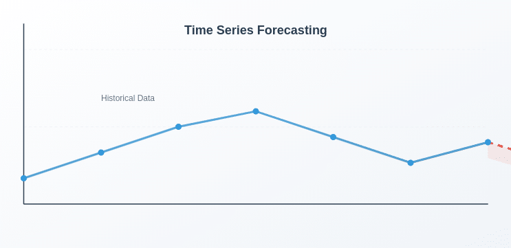
Time Series Forecasting is a predictive modeling that inspects the past data points that have been accumulated over a time period for predicting the future.
Time Series Forecasting is extensively practiced in finance, supply chain planning, weather forecasting, and medical research to foresee trends, recognize patterns, and drive decisions from data.
In contrast to regular predictive analytics, which can emphasize independent variables for predicting an outcome, time series forecasting is actually concerned with sequential, time-based data, in which the observation order is a significant factor.
How Time Series Forecasting Differs from Other Predictive Analytics Techniques?

1. Objective
- Time Series Forecasting: Predicts future values based on historical time-ordered data
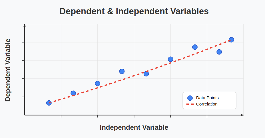
- Regression Analysis: Identifies relationships between independent and dependent variables
- Classification Models: Categorizes data into predefined classes
- Clustering Techniques: Groups similar data points without predefined labels
2. Data Type
- Time Series Forecasting: Sequential, time-dependent data
- Regression Analysis: Independent observations
- Classification Models: Categorical or numerical data
- Clustering Techniques: Unlabeled data
3. Feature Importance
- Time Series Forecasting: Uses past values (lagged variables) and time-dependent patterns
- Regression Analysis: Focuses on explanatory variables
- Classification Models: Relies on feature selection techniques
- Clustering Techniques: Distance-based or similarity measures
4. Dependency on Time
- Time Series Forecasting: Strong (order of data matters)
- Regression Analysis: Weak (order of data does not matter)
- Classification Models: Weak (order of data does not matter)
- Clustering Techniques: No time dependence
5. Common Algorithms
- Time Series Forecasting: ARIMA, Exponential Smoothing, LSTM, Prophet
- Regression Analysis: Linear Regression, Polynomial Regression
- Classification Models: Decision Trees, Random Forest, Neural Networks
- Clustering Techniques: K-Means, DBSCAN, Hierarchical Clustering
6. Application Examples
- Time Series Forecasting: Stock price forecasting, demand prediction, weather forecasting
- Regression Analysis: Sales prediction based on customer demographics
- Classification Models: Spam detection, fraud classification
- Clustering Techniques: Customer segmentation, anomaly detection
Key Components of Time Series Forecasting

1. Trend
A trend represents the complete long-term movement in a time series dataset. It demonstrates whether the data is indicating an upward, downward, or stable pattern over the time.
Types of Trends:
- Upward Trend: A consistent increase in values over time.
Example: The steady rise in global temperatures due to climate change.
- Downward Trend: A continuous decline in values over time.
Example: The decreasing landline telephone subscriptions as mobile phone usage increases.
- Stable (No Trend): Data remains relatively constant with no significant increase or decrease.
Example: Daily energy consumption in an industrial plant with steady operations.
Why Trends Matter in Forecasting?
- Identifying trends helps in making long-term business decisions.
- Ignoring trends can lead to incorrect predictions, especially in industries like finance and e-commerce.
2. Seasonality
Seasonality is about repeating the specific patterns or deviations in the data that are observed at the frequent time intervals, for example, daily, weekly, monthly, or yearly cycles.
Examples of Seasonality:
- Retail Sales: Increased shopping during festivals, Black Friday, & Christmas.
- Weather Patterns: Higher electricity consumption in summers due to air conditioning.
- Website Traffic: More visits to online education platforms at the start of a semester.
Characteristics of Seasonality:
- Fixed & Predictable: Unlike cyclic variations, seasonal patterns repeat over fixed time periods.
- Influences Business Planning: Companies use seasonal trends to plan inventory, marketing campaigns, and staffing.
- Can be Removed for Analysis: Seasonal Adjusted Models help in isolating seasonality to better analyze the underlying trend.
3. Cyclic Patterns
A cyclic pattern shows changes that go up and down over time, but these do not happen on a regular schedule. These changes are often caused by large-scale influences, like economic cycles or shifts in business dynamics.
Unlike seasonal changes, which occur at specific times each year, cyclic variations do not stick to a fixed timeline.
Instead, they rely on outside factors such as how the market is doing, economic changes, or significant global events. These outside factors can make the pattern hard to predict because they do not follow a set path.
Examples of Cyclic Patterns:
- Stock Market: The rise and fall of stock prices based on economic cycles.
- Housing Market: Booms and recessions in real estate, influenced by interest rates and inflation.
- Business Performance: Revenue fluctuations based on industry-wide economic changes.
4. Residuals (Irregular Variations or Noise)
Random noise or residuals are the unforeseen fluctuations in time series data that are not explicitly explainable by trend, seasonality, or cyclic patterns.
Examples of Residuals:
- Stock Market Crashes: Unexpected economic crises causing sharp market drops.
- Natural Disasters: Earthquakes or hurricanes disrupting supply chains and production.
- Viral Social Media Trends: Sudden spikes in traffic due to a viral video or news.
How to Handle Residuals?
- Smoothing Techniques: Methods like moving averages help reduce random fluctuations.
- Anomaly Detection Models: Machine learning models identify outliers caused by unpredictable events.
- Advanced Forecasting Models: Deep learning models (like LSTMs) can capture complex patterns beyond simple trend analysis.
How Time Series Forecasting Works: Step-by-Step Process?

Step 1: Collect and Preprocess Data
Prior to establishing a forecasting model, it is extremely critical to compile high-quality time-series data & clean the same to vacant inconsistencies. Preprocessing makes the model learn based on an orderly dataset.
Key Actions in Data Collection & Preprocessing:
- Data Sources: Time series data can be collected from various sources such as stock market transactions, IoT sensors, sales records, weather stations, economic indicators, and healthcare monitoring systems.
- Handling Missing Values: Missing data can disrupt forecasting accuracy. Common techniques to handle missing values include:
- Forward-fill: Uses the last known value to fill missing entries.
- Backward-fill: Uses the next known value to fill gaps.
- Mean/Median Imputation: Fills missing values using statistical averages.
- Interpolation: Uses mathematical methods to estimate missing points.
- Removing Outliers: Unusual spikes or drops in data may distort the forecast. Methods like Z-score analysis, Interquartile Range (IQR), and Isolation Forests can help detect and remove anomalies.
- Data Transformation for Stationarity: Time series models assume stationarity, meaning the statistical properties (mean, variance) remain constant over time. If the data exhibits non-stationary behavior:
- Differencing can remove trends.
- Box-Cox transformation can stabilize variance.
- Log transformations can reduce the effect of extreme values.
Step 2: Identify Patterns and Components in the Data
Time series data often follows distinct patterns, and identifying them is crucial for choosing an appropriate forecasting model.
Key Components to Analyze:
- Trend: A long-term increase or decrease in the data.
Example: A steady rise in e-commerce sales over the years.
- Seasonality: Recurring patterns at fixed time intervals (daily, weekly, monthly, yearly).
Example: Increased demand for travel bookings during holidays.
- Cyclic Patterns: Long-term fluctuations that do not follow a fixed schedule, often influenced by macroeconomic factors.
Example: Business cycles in the stock market.
- Residuals (Irregular Variations): Unpredictable fluctuations that cannot be explained by trend, seasonality, or cycles.
To visualize these components, tools like time series decomposition (Classical Decomposition, STL Decomposition) can be used.
Step 3: Choose the Right Forecasting Model
Selecting the right model depends on the complexity of patterns in the data, the availability of computational resources, and the forecasting horizon.
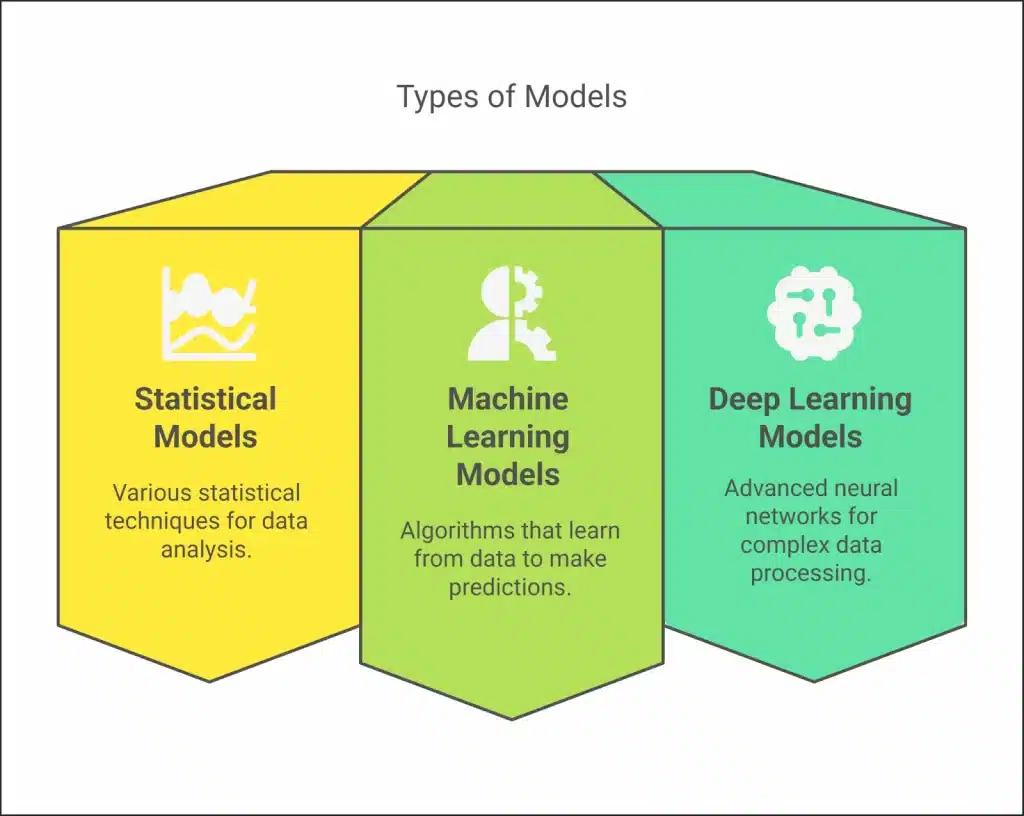
Common Forecasting Models:
Statistical Models:
- ARIMA (AutoRegressive Integrated Moving Average): Suitable for stationary data with trends but no seasonality.
- SARIMA (Seasonal ARIMA): An extension of ARIMA that handles seasonal data patterns.
- Exponential Smoothing (ETS): Useful for data with trends and seasonal variations.
Machine Learning Models:
- Random Forest & XGBoost: Work well when external variables (weather, promotions) affect time series data.
- Support Vector Regression (SVR): Captures non-linear relationships in time series data.
Deep Learning Models:
- LSTMs (Long Short-Term Memory Networks): Ideal for handling long-term dependencies in time series.
- Facebook Prophet: Designed for business forecasting with automated trend and seasonality detection.
Model selection is guided by the characteristics of the data. If the data exhibits simple patterns, ARIMA or ETS might suffice. For complex, multi-variate time series, deep learning models like LSTMs are preferred.
Step 4: Train and Validate the Model
Once the model is selected, it is trained using historical data and validated to check its accuracy.
Key Steps in Training & Validation:
1. Splitting Data into Training and Testing Sets:
- Common ratios: 80% training, 20% testing or 70% training, 30% testing
- Unlike traditional models, time series data must be split chronologically to maintain the time dependency.
2. Cross-Validation in Time Series:
- Rolling Window Validation: The model is trained on past data, and forecasts are tested on the next time window.
- Walk-Forward Validation: The training window expands as new data is added.
3. Hyperparameter Tuning:
- Optimize key parameters such as p, d, q in ARIMA or number of layers in LSTMs using grid search or Bayesian optimization.
Step 5: Evaluate Model Performance
To ensure the model generates reliable forecasts, it must be evaluated using performance metrics.
Common Error Metrics:
- Mean Absolute Error (MAE): Measures average absolute differences between actual and predicted values.
- Mean Squared Error (MSE): Penalizes larger errors by squaring them.
- Root Mean Squared Error (RMSE): More interpretable than MSE as it retains the original unit of measurement.
- Mean Absolute Percentage Error (MAPE): Expresses forecast error as a percentage of actual values, making it easier to interpret across datasets.
If the model performs poorly, revisit feature selection, adjust parameters, or explore advanced models like deep learning-based forecasting.
Step 6: Make Predictions and Interpret Results
Once a model is trained and validated, it is used for forecasting future values.
Key Considerations for Forecasting:
- Short-term vs. Long-term Forecasting:
Short-term forecasts (next few days/weeks) tend to be more accurate than long-term predictions (months/years).
- Generating Prediction Intervals:
Instead of single-point forecasts, models often provide confidence intervals (e.g., 95% confidence) to indicate the range within which future values are likely to fall.
- Visualization of Forecasts:
Line charts, heatmaps, confidence bands, and moving averages are used to present forecast results in an understandable format.
Step 7: Monitor and Improve the Model Over Time
Time series forecasting is not a one-time process. Models need to be monitored and updated continuously to adapt to new trends and data patterns.
Continuous Improvement Strategies:
- Retrain the Model Regularly: Update the model with new data to maintain accuracy.
- Detect Concept Drift: If data distribution changes significantly (due to economic shifts, new business strategies, etc.), retraining may be required.
- Automate Forecasting Pipelines: Use Google AutoML, AWS Forecast, or Python scripts (Prophet, ARIMA, LSTMs) to automate data ingestion, model retraining, and real-time forecasting.
- Deploying Forecasting Models in Production: Time series models can be deployed via cloud-based APIs or embedded into business intelligence (BI) dashboards for real-time decision-making.
Applications Of Time Series Forecasting

1. Demand Forecasting in Retail and E-commerce
- Objective: Predicting customer demand to optimize inventory and supply chain management.
- Application: E-commerce businesses as well as retailers apply time series forecasting to anticipate product demand so that they have the appropriate stock levels. Companies can predict future demand for peak seasons, promotions, and sales events by examining past sales data.
- Example: An e-commerce platform might use time series models to predict the demand for a specific product, ensuring they do not overstock or understock, thus minimizing storage costs and avoiding lost sales.
2. Financial Market Forecasting
- Objective: Predicting stock prices, exchange rates, and financial trends.
- Application: Time series forecasting is extensively employed in finance to forecast stock prices, trends in the stock market, exchange rates, and bond yields. Investors and traders study historical data for the markets to determine trends and forecast future prices so that they can make well-informed decisions.
- Example: A hedge fund could use historical stock price data and ARIMA models to forecast the future movement of a stock, guiding buying or selling decisions.
3. Energy Consumption Forecasting
- Objective: Predicting future energy demand to optimize energy production and distribution.
- Application: Utility companies use time series forecasting to predict energy consumption patterns, ensuring a balance between supply as well as demand. Accurate forecasting helps prevent energy shortages, reduce costs, and improve grid stability.
- Example: A power company might use time series analysis to predict electricity demand during different times of day and seasons, adjusting energy production accordingly to prevent overloading the grid.
4. Weather Forecasting
- Objective: Predicting weather conditions based on historical meteorological data.
- Application: Meteorologists employ time series forecasting to forecast forthcoming weather conditions including temperature, rain, wind speed, as well as storm intensity. Weather forecasting plays an essential role in decision-making for agricultural, aviation, & shipping industries.
- Example: A shipping company may rely on time series forecasting to predict storm patterns and optimize delivery routes, ensuring safety and cost-efficiency.
5. Healthcare and Disease Outbreak Prediction
- Objective: Forecasting disease outbreaks as well as patient volumes to manage healthcare resources.
- Application: Time series prediction in healthcare finds applications in disease outbreaks (flu, COVID-19) & hospitalization forecasts. Reliable projections assists the healthcare administrators control resources, staffing allocation, and preventive procedures.
- Example: Public health agencies as well as hospitals use time series models to predict the spread of infectious diseases, assisting them prepare hospitals with the necessary resources, such as ventilators or vaccines, during peak periods.
Conclusion
Time series forecasting is a key tool used to predict future trends in fields like finance and healthcare. It involves analyzing patterns in data to forecast what might happen next.
Looking to apply these forecasting skills in the real world?
Our Data Science and Machine Learning program, with certification from MIT IDSS, offers hands-on training in predictive analytics. Learn more and build your expertise today!