- What is POS tagging?
- Techniques for POS tagging
- POS tagging with Hidden Markov Model
- Optimizing HMM with Viterbi Algorithm
- Implementation using Python
What is Part of Speech (POS) tagging?
Back in elementary school, we have learned the differences between the various parts of speech tags such as nouns, verbs, adjectives, and adverbs. Associating each word in a sentence with a proper POS (part of speech) is known as POS tagging or POS annotation. POS tags are also known as word classes, morphological classes, or lexical tags.
Back in the days, the POS annotation was manually done by human annotators but being such a laborious task, today we have automatic tools that are capable of tagging each word with an appropriate POS tag within a context.
Nowadays, manual annotation is typically used to annotate a small corpus to be used as training data for the development of a new automatic POS tagger. Annotating modern multi-billion-word corpora manually is unrealistic and automatic tagging is used instead.
POS tags give a large amount of information about a word and its neighbors. Their applications can be found in various tasks such as information retrieval, parsing, Text to Speech (TTS) applications, information extraction, linguistic research for corpora. They are also used as an intermediate step for higher-level NLP tasks such as parsing, semantics analysis, translation, and many more, which makes POS tagging a necessary function for advanced NLP applications.
In this, you will learn how to use POS tagging with the Hidden Makrow model.
Alternatively, you can also follow this link to learn a simpler way to do POS tagging.
If you want to learn NLP, do check out our Free Course on Natural Language Processing at Great Learning Academy.
Techniques for POS tagging
There are various techniques that can be used for POS tagging such as
- Rule-based POS tagging: The rule-based POS tagging models apply a set of handwritten rules and use contextual information to assign POS tags to words. These rules are often known as context frame rules. One such rule might be: “If an ambiguous/unknown word ends with the suffix ‘ing’ and is preceded by a Verb, label it as a Verb”.
- Transformation Based Tagging: The transformation-based approaches use a pre-defined set of handcrafted rules as well as automatically induced rules that are generated during training.
- Deep learning models: Various Deep learning models have been used for POS tagging such as Meta-BiLSTM which have shown an impressive accuracy of around 97 percent.
- Stochastic (Probabilistic) tagging: A stochastic approach includes frequency, probability or statistics. The simplest stochastic approach finds out the most frequently used tag for a specific word in the annotated training data and uses this information to tag that word in the unannotated text. But sometimes this approach comes up with sequences of tags for sentences that are not acceptable according to the grammar rules of a language. One such approach is to calculate the probabilities of various tag sequences that are possible for a sentence and assign the POS tags from the sequence with the highest probability. Hidden Markov Models (HMMs) are probabilistic approaches to assign a POS Tag.
POS tagging with Hidden Markov Model
HMM (Hidden Markov Model) is a Stochastic technique for POS tagging. Hidden Markov models are known for their applications to reinforcement learning and temporal pattern recognition such as speech, handwriting, gesture recognition, musical score following, partial discharges, and bioinformatics.
Let us consider an example proposed by Dr.Luis Serrano and find out how HMM selects an appropriate tag sequence for a sentence.
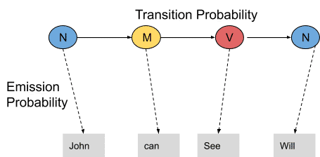
In this example, we consider only 3 POS tags that are noun, model and verb. Let the sentence “ Ted will spot Will ” be tagged as noun, model, verb and a noun and to calculate the probability associated with this particular sequence of tags we require their Transition probability and Emission probability.
The transition probability is the likelihood of a particular sequence for example, how likely is that a noun is followed by a model and a model by a verb and a verb by a noun. This probability is known as Transition probability. It should be high for a particular sequence to be correct.
Now, what is the probability that the word Ted is a noun, will is a model, spot is a verb and Will is a noun. These sets of probabilities are Emission probabilities and should be high for our tagging to be likely.
Let us calculate the above two probabilities for the set of sentences below
- Mary Jane can see Will
- Spot will see Mary
- Will Jane spot Mary?
- Mary will pat Spot
Note that Mary Jane, Spot, and Will are all names.
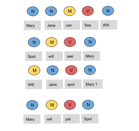
In the above sentences, the word Mary appears four times as a noun. To calculate the emission probabilities, let us create a counting table in a similar manner.
| Words | Noun | Model | Verb |
| Mary | 4 | 0 | 0 |
| Jane | 2 | 0 | 0 |
| Will | 1 | 3 | 0 |
| Spot | 2 | 0 | 1 |
| Can | 0 | 1 | 0 |
| See | 0 | 0 | 2 |
| pat | 0 | 0 | 1 |
Now let us divide each column by the total number of their appearances for example, ‘noun’ appears nine times in the above sentences so divide each term by 9 in the noun column. We get the following table after this operation.
| Words | Noun | Model | Verb |
| Mary | 4/9 | 0 | 0 |
| Jane | 2/9 | 0 | 0 |
| Will | 1/9 | 3/4 | 0 |
| Spot | 2/9 | 0 | 1/4 |
| Can | 0 | 1/4 | 0 |
| See | 0 | 0 | 2/4 |
| pat | 0 | 0 | 1 |
From the above table, we infer that
The probability that Mary is Noun = 4/9
The probability that Mary is Model = 0
The probability that Will is Noun = 1/9
The probability that Will is Model = 3/4
In a similar manner, you can figure out the rest of the probabilities. These are the emission probabilities.
Next, we have to calculate the transition probabilities, so define two more tags <S> and <E>. <S> is placed at the beginning of each sentence and <E> at the end as shown in the figure below.
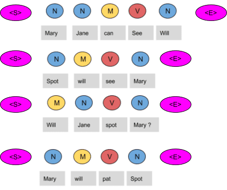
Let us again create a table and fill it with the co-occurrence counts of the tags.
| N | M | V | <E> | |
| <S> | 3 | 1 | 0 | 0 |
| N | 1 | 3 | 1 | 4 |
| M | 1 | 0 | 3 | 0 |
| V | 4 | 0 | 0 | 0 |
In the above figure, we can see that the <S> tag is followed by the N tag three times, thus the first entry is 3.The model tag follows the <S> just once, thus the second entry is 1. In a similar manner, the rest of the table is filled.
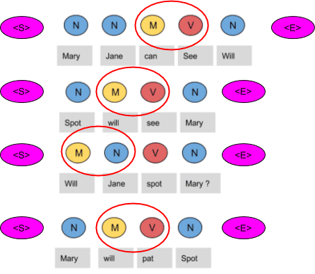
Next, we divide each term in a row of the table by the total number of co-occurrences of the tag in consideration, for example, The Model tag is followed by any other tag four times as shown below, thus we divide each element in the third row by four.
| N | M | V | <E> | |
| <S> | 3/4 | 1/4 | 0 | 0 |
| N | 1/9 | 3/9 | 1/9 | 4/9 |
| M | 1/4 | 0 | 3/4 | 0 |
| V | 4/4 | 0 | 0 | 0 |
These are the respective transition probabilities for the above four sentences. Now how does the HMM determine the appropriate sequence of tags for a particular sentence from the above tables? Let us find it out.
Take a new sentence and tag them with wrong tags. Let the sentence, ‘ Will can spot Mary’ be tagged as-
- Will as a model
- Can as a verb
- Spot as a noun
- Mary as a noun
Now calculate the probability of this sequence being correct in the following manner.
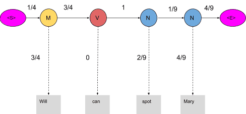
The probability of the tag Model (M) comes after the tag <S> is ¼ as seen in the table. Also, the probability that the word Will is a Model is 3/4. In the same manner, we calculate each and every probability in the graph. Now the product of these probabilities is the likelihood that this sequence is right. Since the tags are not correct, the product is zero.
1/4*3/4*3/4*0*1*2/9*1/9*4/9*4/9=0
When these words are correctly tagged, we get a probability greater than zero as shown below
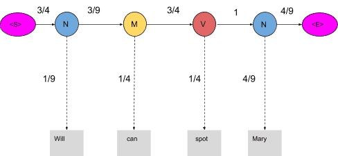
Calculating the product of these terms we get,
3/4*1/9*3/9*1/4*3/4*1/4*1*4/9*4/9=0.00025720164
For our example, keeping into consideration just three POS tags we have mentioned, 81 different combinations of tags can be formed. In this case, calculating the probabilities of all 81 combinations seems achievable. But when the task is to tag a larger sentence and all the POS tags in the Penn Treebank project are taken into consideration, the number of possible combinations grows exponentially and this task seems impossible to achieve. Now let us visualize these 81 combinations as paths and using the transition and emission probability mark each vertex and edge as shown below.
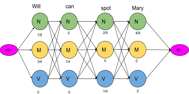
The next step is to delete all the vertices and edges with probability zero, also the vertices which do not lead to the endpoint are removed. Also, we will mention-
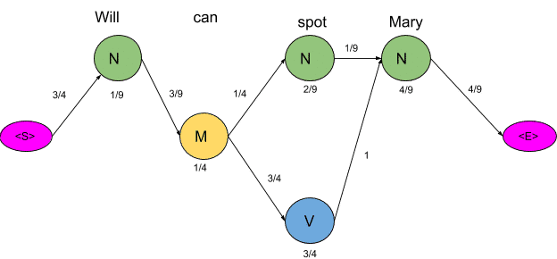
Now there are only two paths that lead to the end, let us calculate the probability associated with each path.
<S>→N→M→N→N→<E> =3/4*1/9*3/9*1/4*1/4*2/9*1/9*4/9*4/9=0.00000846754
<S>→N→M→N→V→<E>=3/4*1/9*3/9*1/4*3/4*1/4*1*4/9*4/9=0.00025720164
Clearly, the probability of the second sequence is much higher and hence the HMM is going to tag each word in the sentence according to this sequence.
Optimizing HMM with Viterbi Algorithm
The Viterbi algorithm is a dynamic programming algorithm for finding the most likely sequence of hidden states—called the Viterbi path—that results in a sequence of observed events, especially in the context of Markov information sources and hidden Markov models (HMM).
Source: Wikipedia
In the previous section, we optimized the HMM and bought our calculations down from 81 to just two. Now we are going to further optimize the HMM by using the Viterbi algorithm. Let us use the same example we used before and apply the Viterbi algorithm to it.
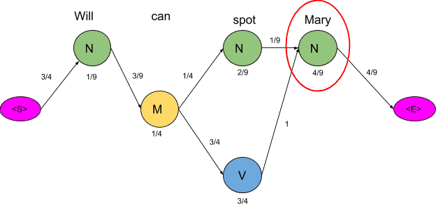
Consider the vertex encircled in the above example. There are two paths leading to this vertex as shown below along with the probabilities of the two mini-paths.
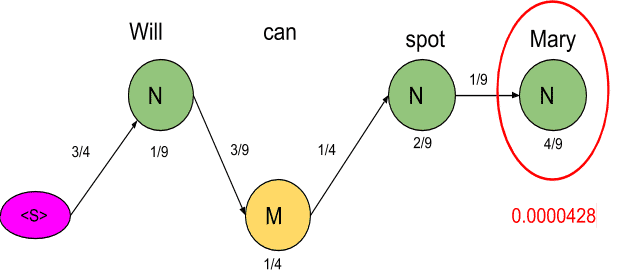
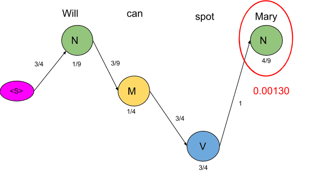
Now we are really concerned with the mini path having the lowest probability. The same procedure is done for all the states in the graph as shown in the figure below
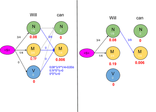
As we can see in the figure above, the probabilities of all paths leading to a node are calculated and we remove the edges or path which has lower probability cost. Also, you may notice some nodes having the probability of zero and such nodes have no edges attached to them as all the paths are having zero probability. The graph obtained after computing probabilities of all paths leading to a node is shown below:
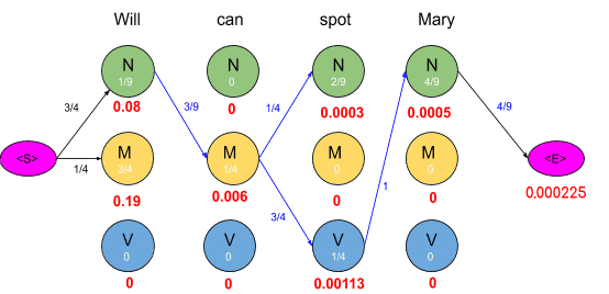
To get an optimal path, we start from the end and trace backward, since each state has only one incoming edge, This gives us a path as shown below
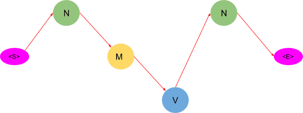
As you may have noticed, this algorithm returns only one path as compared to the previous method which suggested two paths. Thus by using this algorithm, we saved us a lot of computations.
After applying the Viterbi algorithm the model tags the sentence as following-
- Will as a noun
- Can as a model
- Spot as a verb
- Mary as a noun
These are the right tags so we conclude that the model can successfully tag the words with their appropriate POS tags.
Implementation using Python
In this section, we are going to use Python to code a POS tagging model based on the HMM and Viterbi algorithm.
# Importing libraries
import nltk
import numpy as np
import pandas as pd
import random
from sklearn.model_selection import train_test_split
import pprint, time

#download the treebank corpus from nltk
nltk.download('treebank')

#download the universal tagset from nltk
nltk.download('universal_tagset')

# reading the Treebank tagged sentences
nltk_data = list(nltk.corpus.treebank.tagged_sents(tagset='universal'))

#print the first two sentences along with tags
print(nltk_data[:2])
Output:

#print each word with its respective tag for first two sentences
for sent in nltk_data[:2]:
  for tuple in sent:
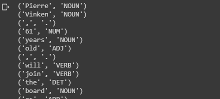
    print(tuple)
Output:
# split data into training and validation set in the ratio 80:20
train_set,test_set =train_test_split(nltk_data,train_size=0.80,test_size=0.20,random_state = 101)
# create list of train and test tagged words
train_tagged_words = [ tup for sent in train_set for tup in sent ]
test_tagged_words = [ tup for sent in test_set for tup in sent ]
print(len(train_tagged_words))
print(len(test_tagged_words))
Output:

# check some of the tagged words.
train_tagged_words[:5]
Output:

#use set datatype to check how many unique tags are present in training data
tags = {tag for word,tag in train_tagged_words}
print(len(tags))
print(tags)

# check total words in vocabulary
vocab = {word for word,tag in train_tagged_words}
Output:

# compute Emission Probability
def word_given_tag(word, tag, train_bag = train_tagged_words):
    tag_list = [pair for pair in train_bag if pair[1]==tag]
    count_tag = len(tag_list)#total number of times the passed tag occurred in train_bag
    w_given_tag_list = [pair[0] for pair in tag_list if pair[0]==word]
#now calculate the total number of times the passed word occurred as the passed tag.
    count_w_given_tag = len(w_given_tag_list)


    return (count_w_given_tag, count_tag)
# compute  Transition Probability
def t2_given_t1(t2, t1, train_bag = train_tagged_words):
    tags = [pair[1] for pair in train_bag]
    count_t1 = len([t for t in tags if t==t1])
    count_t2_t1 = 0
    for index in range(len(tags)-1):
        if tags[index]==t1 and tags[index+1] == t2:
            count_t2_t1 += 1
    return (count_t2_t1, count_t1)
# creating t x t transition matrix of tags, t= no of tags
# Matrix(i, j) represents P(jth tag after the ith tag)

tags_matrix = np.zeros((len(tags), len(tags)), dtype='float32')
for i, t1 in enumerate(list(tags)):
    for j, t2 in enumerate(list(tags)):
        tags_matrix[i, j] = t2_given_t1(t2, t1)[0]/t2_given_t1(t2, t1)[1]

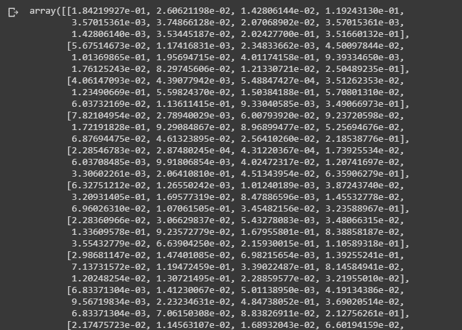
print(tags_matrix)
Output:
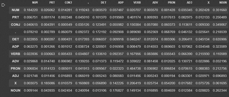
# convert the matrix to a df for better readability
#the table is same as the transition table shown in section 3 of article
tags_df = pd.DataFrame(tags_matrix, columns = list(tags), index=list(tags))
display(tags_df)
Output:
def Viterbi(words, train_bag = train_tagged_words):
    state = []
    T = list(set([pair[1] for pair in train_bag]))

    for key, word in enumerate(words):
        #initialise list of probability column for a given observation
        p = []
        for tag in T:
            if key == 0:
                transition_p = tags_df.loc['.', tag]
            else:
                transition_p = tags_df.loc[state[-1], tag]

            # compute emission and state probabilities
            emission_p = word_given_tag(words[key], tag)[0]/word_given_tag(words[key], tag)[1]
            state_probability = emission_p * transition_p
            p.append(state_probability)

        pmax = max(p)
        # getting state for which probability is maximum
        state_max = T[p.index(pmax)]
        state.append(state_max)
    return list(zip(words, state))
# Let's test our Viterbi algorithm on a few sample sentences of test dataset
random.seed(1234)      #define a random seed to get same sentences when run multiple times

# choose random 10 numbers
rndom = [random.randint(1,len(test_set)) for x in range(10)]

# list of 10 sents on which we test the model
test_run = [test_set[i] for i in rndom]

# list of tagged words
test_run_base = [tup for sent in test_run for tup in sent]

# list of untagged words
test_tagged_words = [tup[0] for sent in test_run for tup in sent]
#Here We will only test 10 sentences to check the accuracy
#as testing the whole training set takes huge amount of time
start = time.time()
tagged_seq = Viterbi(test_tagged_words)
end = time.time()
difference = end-start

print("Time taken in seconds: ", difference)

# accuracy
check = [i for i, j in zip(tagged_seq, test_run_base) if i == j]

accuracy = len(check)/len(tagged_seq)
print('Viterbi Algorithm Accuracy: ',accuracy*100)
Output:

#Code to test all the test sentences
#(takes alot of time to run s0 we wont run it here)
# tagging the test sentences()
test_tagged_words = [tup for sent in test_set for tup in sent]
test_untagged_words = [tup[0] for sent in test_set for tup in sent]
test_untagged_words

start = time.time()
tagged_seq = Viterbi(test_untagged_words)
end = time.time()
difference = end-start

print("Time taken in seconds: ", difference)

# accuracy
check = [i for i, j in zip(test_tagged_words, test_untagged_words) if i == j]

accuracy = len(check)/len(tagged_seq)
print('Viterbi Algorithm Accuracy: ',accuracy*100)
#To improve the performance,we specify a rule base tagger for unknown words
# specify patterns for tagging
patterns = [
    (r'.*ing$', 'VERB'),              # gerund
    (r'.*ed$', 'VERB'),               # past tense
    (r'.*es$', 'VERB'),               # verb
    (r'.*\'s$', 'NOUN'),              # possessive nouns
    (r'.*s$', 'NOUN'),                # plural nouns
    (r'\*T?\*?-[0-9]+$', 'X'),        # X
    (r'^-?[0-9]+(.[0-9]+)?$', 'NUM'), # cardinal numbers
    (r'.*', 'NOUN')                   # nouns
]

# rule based tagger
rule_based_tagger = nltk.RegexpTagger(patterns)
#modified Viterbi to include rule based tagger in it
def Viterbi_rule_based(words, train_bag = train_tagged_words):
    state = []
    T = list(set([pair[1] for pair in train_bag]))

    for key, word in enumerate(words):
        #initialise list of probability column for a given observation
        p = []
        for tag in T:
            if key == 0:
                transition_p = tags_df.loc['.', tag]
            else:
                transition_p = tags_df.loc[state[-1], tag]

            # compute emission and state probabilities
            emission_p = word_given_tag(words[key], tag)[0]/word_given_tag(words[key], tag)[1]
            state_probability = emission_p * transition_p
            p.append(state_probability)

        pmax = max(p)
        state_max = rule_based_tagger.tag([word])[0][1]


        if(pmax==0):
            state_max = rule_based_tagger.tag([word])[0][1] # assign based on rule based tagger
        else:
            if state_max != 'X':
                # getting state for which probability is maximum
                state_max = T[p.index(pmax)]


        state.append(state_max)
    return list(zip(words, state))
#test accuracy on subset of test data
start = time.time()
tagged_seq = Viterbi_rule_based(test_tagged_words)
end = time.time()
difference = end-start

print("Time taken in seconds: ", difference)

# accuracy
check = [i for i, j in zip(tagged_seq, test_run_base) if i == j]

accuracy = len(check)/len(tagged_seq)
print('Viterbi Algorithm Accuracy: ',accuracy*100)
Output:

#Check how a sentence is tagged by the two POS taggers
#and compare them
test_sent="Will can see Marry"
pred_tags_rule=Viterbi_rule_based(test_sent.split())
pred_tags_withoutRules= Viterbi(test_sent.split())
print(pred_tags_rule)
print(pred_tags_withoutRules)
#Will and Marry are tagged as NUM as they are unknown words for Viterbi Algorithm
Output:

As seen above, using the Viterbi algorithm along with rules can yield us better results.
This brings us to the end of this article where we have learned how HMM and Viterbi algorithm can be used for POS tagging.
If you wish to learn more about Python and the concepts of ML, upskill with Great Learning’s PG Program Artificial Intelligence and Machine Learning.


