Are Your Machine Learning Models Really Smart? 🤔
Ever trained a model that performs amazingly on training data but fails miserably on new data? That’s where Overfitting and Underfitting come in! These two problems can make or break your machine learning model’s ability to generalize.
In this article, we’ll break down these concepts, understand why they happen, and explore effective techniques to fix them. Let’s dive in!
Understanding Model Performance: Overfitting vs. Underfitting
Whenever we train a machine learning model, we aim to create a system that can accurately predict outcomes for new, unseen data. To evaluate a model’s performance, we typically split our dataset into:
- Training Set: Used to train the model.
- Testing Set: Used to evaluate how well the model generalizes.
Sometimes, despite following a structured training process, our model fails to make accurate predictions. This happens due to either underfitting or overfitting of the data. Let’s analyze these two scenarios in detail.
What is Underfitting?

Underfitting occurs when a model is too simple to capture the underlying patterns in the training data. In other words, the model has high bias and fails to learn the relationships between input features and output labels effectively.
Characteristics of Underfitting:
- The model performs poorly on both training and test datasets.
- It fails to capture the complexity of the dataset.
- Adding more training data does not improve performance significantly.
- It occurs when models are too simple (e.g., using linear regression for a non-linear dataset).

Example of Underfitting:
Consider a dataset where you want to predict house prices based on square footage. If you apply a simple linear regression model to this data when the relationship is actually quadratic or exponential, the model will struggle to provide accurate predictions. The result is underfitting, where the model is too simple to grasp the underlying trend.
What is Overfitting?
Overfitting occurs when a model learns the training data too well, including its noise and irrelevant details. Instead of generalizing patterns, the model memorizes the data, leading to poor performance on unseen test data. This happens due to high variance in the model.

Characteristics of Overfitting:
- The model performs exceptionally well on training data but poorly on test data.
- It captures noise and anomalies instead of general patterns.
- The model has too many parameters and is overly complex.
- It fails to generalize well to new datasets.

Example of Overfitting:
Imagine training a deep neural network on a dataset of handwritten digits. If the model is excessively complex, it might memorize the exact pixel patterns of each image instead of learning general features like stroke patterns and curves. As a result, when tested on new handwritten digits, it may struggle to recognize them correctly.
Also Read: What is a Neural Network?
The Bias-Variance Tradeoff
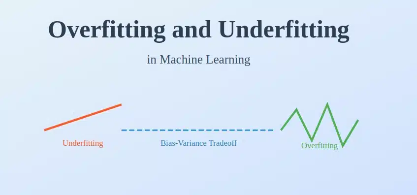
The bias-variance tradeoff explains why underfitting and overfitting occur. It represents the relationship between a model’s complexity and its ability to generalize well.
- High Bias (Underfitting): The model makes strong assumptions about the data and fails to capture patterns.
- High Variance (Overfitting): The model is too sensitive to small fluctuations in the data, leading to poor generalization.
A well-balanced model should achieve an optimal balance between bias and variance, ensuring it captures the necessary patterns without memorizing noise.
How to Identify Overfitting and Underfitting
The best way to detect whether a model is underfitting or overfitting is by evaluating its performance on training and test datasets.
- Underfitting: Low accuracy on both training and test sets.
- Overfitting: High accuracy on the training set but significantly lower accuracy on the test set.

Graphical Representation
- Underfitting (High Bias): The model’s prediction line does not cover all data points.
- Overfitting (High Variance): The model’s prediction line fits the training data perfectly, including noise and outliers.
- Good Fit: The model’s prediction line captures the trend while avoiding excessive complexity.
Techniques to Overcome Underfitting and Overfitting
Now that we understand the causes of underfitting and overfitting, let’s explore techniques to mitigate them.
How to Overcome Underfitting

- Increase Model Complexity – Use more complex models, such as polynomial regression instead of simple linear regression.
- Add More Features – Include additional relevant input features to improve learning.
- Reduce Regularization – If regularization is too strong (e.g., high L1/L2 penalties), it may overly simplify the model.
- Train for a Longer Time – Some models require more training epochs to learn patterns effectively.
How to Overcome Overfitting

- Regularization Techniques:
- L1 Regularization (Lasso Regression): Helps reduce complexity by setting some feature weights to zero.
- L2 Regularization (Ridge Regression): Shrinks feature weights without setting them to zero.
- Elastic Net: A combination of L1 and L2 regularization.
- Cross-Validation:
- Use k-fold cross-validation to ensure that the model generalizes well across different data subsets.
- Pruning Decision Trees:
- In decision trees, reduce the depth to prevent over-complexity.
- Dropout in Neural Networks:
- Randomly drop some neurons during training to prevent over-reliance on specific patterns.
- Increase Training Data:
- More data helps the model generalize better and avoid learning noise.
- Early Stopping:
- Stop training when validation loss starts increasing to prevent memorization.
Learn how Alpha-Beta Pruning in AI optimizes decision-making in game theory by reducing the number of nodes evaluated in the minimax algorithm.
Real-World Applications
Overfitting and underfitting are crucial concerns across various domains:

- Healthcare: Predicting diseases based on medical data requires generalizable models.
- Finance: Stock market predictions should avoid memorizing past fluctuations.
- Autonomous Vehicles: Object detection systems must generalize across diverse environments.
- Natural Language Processing: Sentiment analysis models should not memorize specific training phrases.
Conclusion
Achieving a balance between underfitting and overfitting is key to building robust machine learning models. While underfitting leads to poor learning due to excessive simplification, overfitting results in poor generalization due to unnecessary complexity.
By understanding the bias-variance tradeoff and applying techniques like regularization, cross-validation, dropout, and pruning, we can develop models that perform well on both training and unseen test data.
Machine learning practitioners must always strive to optimize their models to achieve a good fit, ensuring high accuracy and reliability in real-world applications.
Advance your career with the PG Program in Artificial Intelligence. Gain expertise in AI, Machine Learning, Neural Networks, and Deep Learning through industry-relevant projects and expert mentorship.
Frequently Asked Questions
How does feature selection help in preventing overfitting?
Feature selection removes irrelevant or redundant features, reducing noise and improving model generalization, thus preventing overfitting.
Can ensemble methods help reduce overfitting and underfitting?
Yes, ensemble methods like bagging (reduces variance) and boosting (reduces bias) improve model performance by combining multiple models.
Also Read: Bagging and Boosting
Why do deep learning models overfit easily?
Deep learning models have many parameters, making them prone to memorizing training data instead of learning general patterns. Regularization and dropout help mitigate this.
What role does batch size play in overfitting and underfitting?
Small batch sizes introduce noise, improving generalization, while large batches may lead to overfitting by memorizing patterns too well.
How can transfer learning help with overfitting and underfitting?
Transfer learning applies pre-trained models to new tasks, reducing overfitting by leveraging learned features and preventing underfitting with better feature extraction.


