Multinomial Logistic Regression is similar to logistic regression but with a difference, that the target dependent variable can have more than two classes i.e. multiclass or polychotomous.
For example, the students can choose a major for graduation among the streams “Science”, “Arts” and “Commerce”, which is a multiclass dependent variable and the independent variables can be marks, grade in competitive exams, Parents profile, interest etc.
What is Multinomial Logistic Regression?
Multinomial Logistic Regression is a classification technique that extends the logistic regression algorithm to solve multiclass possible outcome problems, given one or more independent variables.
This model is used to predict the probabilities of categorically dependent variable, which has two or more possible outcome classes. Whereas the logistic regression model is used when the dependent categorical variable has two outcome classes for example, students can either “Pass” or “Fail” in an exam or bank manager can either “Grant” or “Reject” the loan for a person.Check out the logistic regression algorithm course and understand this topic in depth.
Example for Multinomial Logistic Regression:
(a) Which Flavor of ice cream will a person choose?
Dependent Variable:
- Vanilla
- Chocolate
- Butterscotch
- Black Current
Independent Variables:
- Gender
- Age
- Occasion
- Happiness
- Etc.
Multinomial Logistic Regression is also known as multiclass logistic regression, softmax regression, polytomous logistic regression, multinomial logit, maximum entropy (MaxEnt) classifier and conditional maximum entropy model.
Dependent Variable:
The dependent Variable can have two or more possible outcomes/classes.
The dependent variables are nominal in nature means there is no any kind of ordering in target dependent classes i.e. these classes cannot be meaningfully ordered.
The dependent variable to be predicted belongs to a limited set of items defined.
Assumptions:
When you want to choose multinomial logistic regression as the classification algorithm for your problem, then you need to make sure that the data should satisfy some of the assumptions required for multinomial logistic regression.
- The Dependent variable should be either nominal or ordinal variable.
Nominal variable is a variable that has two or more categories but it does not have any meaningful ordering in them. For example, (a) 3 types of cuisine i.e. Indian, Continental and Italian. (b) 5 categories of transport i.e. Bus, Car, Train, Ship and Airplane.
Ordinal variable are variables that also can have two or more categories but they can be ordered or ranked among themselves. For example, Grades in an exam i.e. A-excellent, B-Good, C-Needs Improvement and D-Fail. When ordinal dependent variable is present, one can think of ordinal logistic regression.
- Set of one or more Independent variables can be continuous, ordinal or nominal.
Continuous variables are numeric variables that can have infinite number of values within the specified range values. For example, age of a person, number of hours students study, income of an person.
Ordinal variables should be treated as either continuous or nominal.
- The Observations and dependent variables must be mutually exclusive and exhaustive.
Mutually exclusive means when there are two or more categories, no observation falls into more than one category of dependent variable.
The categories are exhaustive means that every observation must fall into some category of dependent variable.
- No Multicollinearity between Independent variables.
Multicollinearity occurs when two or more independent variables are highly correlated with each other. This makes it difficult to understand how much every independent variable contributes to the category of dependent variable. Also makes it difficult to understand the importance of different variables.
- There should be no Outliers in the data points.
Solution Approaches:
- K models for K classes.
This is the simplest approach where k models will be built for k classes as a set of independent binomial logistic regression.
For Example, there are three classes in nominal dependent variable i.e., A, B and C. Firstly, Build three models separately i.e. Class A vs Class B & C, Class B vs Class A & C and Class C vs Class A & B.
During First model, (Class A vs Class B & C): Class A will be 1 and Class B&C will be 0. In second model (Class B vs Class A & C): Class B will be 1 and Class A&C will be 0 and in third model (Class C vs Class A & B): Class C will be 1 and Class A&B will be 0.
Next develop the equation to calculate three Probabilities i.e. P(A), P(B) and P(C), very similar to the logistic regression equation.

Predicting the class of any record/observations, based on the independent input variables, will be the class that has highest probability. For a record, if P(A) > P(B) and P(A) > P(C), then the dependent target class = Class A.
- Simultaneous Models.
For K classes/possible outcomes, we will develop K-1 models as a set of independent binary regressions, in which one outcome/class is chosen as “Reference/Pivot” class and all the other K-1 outcomes/classes are separately regressed against the pivot outcome.
When K = two, one model will be developed and multinomial logistic regression is equal to logistic regression.
For two classes i.e. Class A and Class B, one logistic regression model will be developed and the equation for probability is as follows:

If the value of p >= 0.5, then the record is classified as class A, else class B will be the possible target outcome.
For Multi-class dependent variables i.e. for K classes, K-1 Logistic Regression models will be developed. Let’s say there are three classes in dependent variable/Possible outcomes i.e. Class A, B and C.
Since there are three classes, two logistic regression models will be developed and let’s consider Class C has the reference or pivot class.
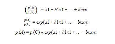
First Model will be developed for Class A and the reference class is C, the probability equation is as follows:

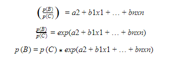
Develop second logistic regression model for class B with class C as reference class, then the probability equation is as follows:


Once probability of class C is calculated, probabilities of class A and class B can be calculated using the earlier equations.
Same logic can be applied to k classes where k-1 logistic regression models should be developed.
There are other approaches for solving the multinomial logistic regression problems.
Advantages:
– Helps to understand the relationships among the variables present in the dataset.
– Simultaneous Models result in smaller standard errors for the parameter estimates than when fitting the logistic regression models separately.
– The choice of reference class has no effect on the parameter estimates for other categories.
This brings us to the end of the blog on Multinomial Logistic Regression. We hope that you enjoyed this and were able to gain some insights, check out Great Learning Academy’s pool of Free Online Courses and upskill today!
Contributed by: Keerthana V


