

In every algorithm of machine learning, there is an approach that is unique yet easily interpretable. Logistic regression is one such algorithm with an easy and unique approach. It is very often used in the credit and risk industry for its easy intuition on predicting the chances of default and risk cases. It is indeed quite a challenge to break down most of the algorithms due to their black-box nature and their hard to find parameters, but logistic regression outperforms all. So it is time to break down the entire algorithm and draw some inferences.
We can say that logistic regression solely depends on maximum likelihood estimation. Now let us focus on this and after that, we will jump back to the core concepts including parameters. Learn more about the Logistic regression algorithm here.
Maximum likelihood estimation maximises the probability that classifies the event being 1 or 0 by estimating certain parameters. Every probability equation goes by the following.
probability (event + non-event) = 1
Logistic regression is capable of finding out the probability only after transforming the dependent variable into a logit variable with respect to the independent variable or the features present in the data.
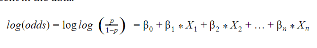
The reason being using log function is to increase the range of probability of classification of events. Let us explain how it works.
Range of Probability = [0,1]
Range of Odds = [0, + ∞] as Odds = (Probability)/(1-Probability)
Range of log(odds) = [- ∞, + ∞]
Here as we can see how the range of [0,1] increased to [-,+] which is what we wanted.
Now the entire mechanism behind the logistic regression has been covered, let us break further to the terminologies involved in it.
Information Value
This parameter is considered even before building the model. This is useful in eliminating those variables which seem to be weak for prediction and is considered a weak contributor to the dependent variable. Let us understand the following equation.
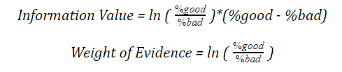
Now this equation seems to be tricky at first, so let us go with an example and get a clear idea of how it works.
The bins given above are the price range followed by the events and non-events. After we calculated the information value, we found a value of 0.0356 which is 3.5% and we can say it is a weak predictor as it contributes only 3.5% to the dependent variable.
Let us see the predictive power of the variables based on their information value
| Information Value | Predictive Power |
| < 0.02 | Useless of prediction |
| 0.02 – 0.1 | Weak Predictor |
| 0.1 – 0.3 | Medium Predictor |
| 0.3 – 0.5 | Strong Predictor |
| > 0.5 | Suspicious or too good Predictor |
Also Read: Linear Regression in Machine Learning
Akaike Information Criteria
This parameter helps us to find the relatedness of our model by acting as a tradeoff between bias and variance.
Key point – The lower the AIC the better is the model.
AIC can be calculated by the following equation
AIC = -2*ln(L) + 2*k
L = Maximum value of Likelihood (log transformation applied for mathematical convenience)
k = number of variables in the model
Here the parameter k is used to penalise the overfitting issue in a model.
ROC Curve
ROC or Receiver Operating Characteristics curve is a graphical representation of the performance of a binary classification model. It shows the variation between True positive and False positive rate at different threshold values.
The ROC curve can give us a clear idea to set a threshold value to classify the label and also help in model optimisation.
A low threshold value we will put most of the predicted observations under the positive category, even when some of them should be placed under the negative category. On the other hand, keeping the threshold at a very high level penalises the positive category, but the negative category will improve.
For such case an optimum threshold value can give a better accuracy which can be found on ROC curve
ROC curve will look as follow:
To gain more information on sensitivity and specificity, we need to go through the following formula.
Recall (Sensitivity or TPR) = TP/(TP+FN)
Specificity (TNR) = TN/(FP+TN)
Evaluation parameters
Following are the evaluation parameters considered in logistic regression
- Precision
- Recall
- F1-Score
- ROC curve
All the above parameters are considered on positive and negative rates of the classes which are tabulated below
| Predicted: YES | Predicted: NO | |
| Actual: YES | TP ( True Positive) | FN ( True Positive) |
| Actual: NO | FP ( True Positive) | TN ( True Positive) |
(a) Precision: Precision is an evaluation measure which is the combination of relevant as well as retrieved items over the total number of retrieved results. It is basically used when the case of false-positive prediction is high.
Precision (TNR) = TPTP+FP
b) Recall: Recall is a measure when False negative is considered.
Recall (Sensitivity or TPR) = TP/(TP+FN)
c) ROC Curve (Explained above)
d)F1-Score: F1-Score is an evaluation technique that maintains a balance between precision and recall.
F1 Score = 2 * (Precision*Recall)/(Precision+Recall)
Now in some cases precision and recall can be a dangerous call. Let us understand that further.
Precision and recall are two of the evaluation techniques used in a machine learning model which tells us how better a model can perform. But there are certain business domains where these two evaluation techniques can cause a business risk.
Medical Industry
Let us suppose we are analysing the records of patients suffering from cancer and we are trying to predict whether the upcoming patients will suffer from cancer or not. Now, the precision is considered when the false positive rates are high which means the patient is not suffering from cancer but the machine predicts as a cancer patient.
In case of recall, false negatives are high which means the patient is suffering from cancer and the model predicts the patient as cancer-free.
| Cancer patients | Predicted: Yes (Having cancer) | Predicted: No (Not having cancer) |
| Actual: Yes (Having cancer) | 90 | 10 |
| Actual: No (Not having cancer) | 80 | 20 |
Accuracy of the model= (90+20)/200=0.55
Precision of the model=90/(90+80)=0.53
Recall of the model=90/(90+10)=0.9
Now the model is 55% accurate but if we see the recall, then it is 90% accurate. But if we consider recall as accuracy then it will declare many patients as cancer-free although they are suffering from cancer.
Banking Sector
In the banking sector, let us assume building a model to check whether a customer is eligible for a loan or not. Let us again build a model on 200 customers and evaluate based on accuracy, precision and recall. Check out this Logistic regression on customer data
course.
| Customer | Predicted: Yes (Eligible for a loan) | Predicted: No (Not eligible) |
| Actual: Yes (Eligible for a loan) | 80 | 20 |
| Actual: No (Not eligible) | 8 | 92 |
Accuracy of the model= (80+92)/200=0.86
Precision of the model=80/(80+8)=0.9
Recall of the model=80/(80+20)=0.8
Now the model is 86% accurate but if we consider the precision we see it is 90%. Now if we evaluate the model by precision, then there is a high chance that a person is not eligible for loan but the bank is sanctioning loan for them. In that case, the bank may incur huge losses.
Precision works fine when false-positive cases are high. On the other hand, recall works fine when false-negative cases are high. Many domains such as medical, educational or legal fields are delicate, where evaluating entities with such measures can cost more risk. In such cases, F1-Score performs better as it is the only measure that maintains a balance between precision and recall.
F1-Score is the harmonic mean of precision and recall. Multiplying the constant of 2 scales the score to 1 when both precision and recall are 1.
In such cases, F1-score can be a good evaluation technique because it maintains a balance between precision and recall and can tell almost exactly whether a person is eligible for a loan or not.
The best evaluation technique is accuracy which can tell us the best prediction because it gives the ratio of true prediction to total actual values.
Accuracy = TP+TNTP+FN+TN+FP
Merits of Logistic Regression
- Logistic Regression has less chance of overfitting
- It is much easier to implement compared to other algorithms
- Tuning of parameters is not required much
Demerits of Logistic Regression
- They fail to play good in large datasets
- The algorithm only works fine in linearly separable data
- They are not flexible with continuous data
Applications of Logistic Regression
Logistic regression is a well-applied algorithm that is widely used in many sectors. Some of them are:
Medical sector
Logistic regression is mostly used to analyse the risk of patients suffering from various diseases. Also, it can predict the risk of various diseases that are difficult to treat.
Banking sector
Logistic regression is one of the most used algorithms in banking sectors as we can set various threshold values to expect the probabilities of a person eligible for loan or not. Also, they play a huge role in analysing credit and risk of fraudulent activities in the industry.
Example of Logistic Regression in Python
Now let us take a case study in Python. We will be taking data from social network ads which tell us whether a person will purchase the ad or not based on the features such as age and salary.
First, we will import all the libraries:
import numpy as np
import matplotlib.pyplot as plt
import pandas as pd
Now we will import the dataset and select only age and salary as the features
dataset = pd.read_csv('Social_Network_Ads.csv')
dataset.head()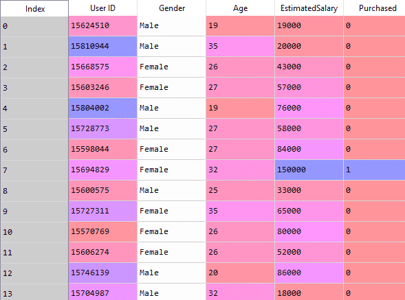
X = dataset.iloc[:, [2, 3]].values
y = dataset.iloc[:, 4].values
Now we will perform splitting for training and testing. We will take 75% of the data for training, and test on the remaining data
from sklearn.model_selection  import train_test_split
X_train, X_test, y_train, y_test = train_test_split(X, y, test_size = 0.25, random_state = 0)
Next, we scale the features to avoid variation and let the features follow a normal distribution
from sklearn.preprocessing import StandardScaler
sc = StandardScaler()
X_train = sc.fit_transform(X_train)
X_test = sc.transform(X_test)
The preprocessing part is over. It is time to fit the model
from sklearn.linear_model import LogisticRegression
classifier = LogisticRegression(random_state = 0)
classifier.fit(X_train, y_train)
We fitted the model on training data. We will predict the labels of test data.
y_pred = classifier.predict(X_test)The prediction is over. Now we will evaluate the performance of our model.
From sklearn.metrics import confusion_matrix,classification_report
cm = confusion_matrix(y_test, y_pred)
cl_report=classification_report(y_test,y_pred)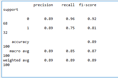
Now we can see that our model performed really good based on precision and recall.
Example of Logistic Regression in R
We will perform the application in R and look into the performance as compared to Python
First, we will import the dataset
dataset = read.csv('Social_Network_Ads.csv')
We will select only Age and Salary
dataset = dataset [3:5]
Now we will encode the target variable as a factor
dataset$Purchased = factor (dataset$Purchased, levels = c (0, 1))Next, we will split the data into training and testing.
# install.packages('caTools')
library(caTools)
set.seed(123)
split = sample.split(dataset$Purchased, SplitRatio = 0.75)
training_set = subset (dataset, split == TRUE)
test_set = subset (dataset, split == FALSE)
Then we will perform scaling only on the feature variables
training_set[-3] = scale(training_set[-3])
test_set[-3] = scale(test_set[-3])
After preprocessing is done, we will fit the model and get ready for prediction
# Fitting Logistic Regression to the Training set
classifier = glm(formula = Purchased ~ .,
                 family = binomial,
                 data = training_set)
The fitting is done. Now we predict the values by keeping the threshold as 0.5. It means that the probability above 0.5 is counted as 1 and the rest as 0.
prob_pred = predict (classifier, type = 'response', newdata = test_set[-3])
y_pred = ifelse (prob_pred > 0.5, 1, 0)
Now we will evaluate our model based on the confusion matrix and make a comparison with Python.
cm = table (test_set[, 3], y_pred > 0.5)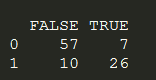
As we see the rate of misclassification is much higher in R than in Python. But we can only challenge it when the data splitting will be the same in both cases.
Conclusion
Logistic Regression works fine only when the target variable is discrete in nature. They do not have the flexibility to act as regression analysis. Also, they have less chance of overfitting but in data having a higher dimension, logistic can overfit. For such cases, there are regularising techniques called L1 and L2 which shrink the coefficients of the algorithm to avoid overfitting. Logistic regression can also work fine with the discretised data as they do not follow a decision-based approach. Learn more with the help of a logistic regression course. Join now!