The interest in Computer Vision has seen a tremendous spike in the last decade credit to the endless applications it offers. Vision is a key sense for Human beings. Thus, equipping Machines with the ability to perform tasks that earlier only Human Systems could do, has opened doors to achieve automation in various fields such as Healthcare, Agriculture, Logistics, and many more.
Before starting the discussion on Fully Convolutional Layer (FCNs from now on), let us set up the context by understanding the application and why there was a need to implement FCN in the first place.
Contributed by: Rahul Purohit
Computer Vision tasks can be broadly categorized into Four Types –
1. Classification
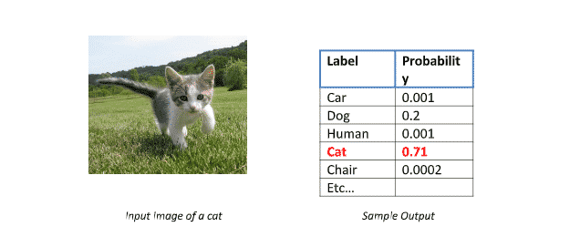
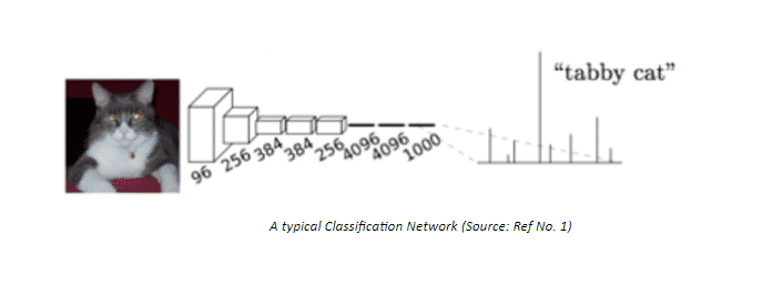
A typical classification problem aims to identify (and or localize) an object in an input image. We usually have a single point of interest in such problems, and thus the output is a vector of probabilities of different classes present in the training corpus. The subject is classified into the class label having the maximum value of probability.
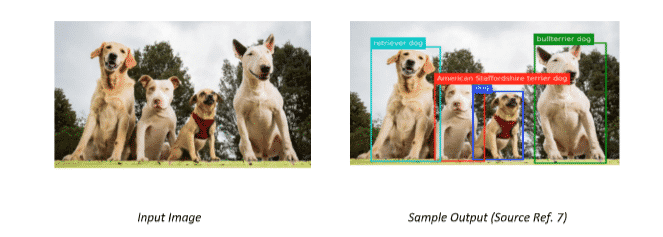
2. Object Detection
Object detection is a computer vision task that identifies and locate objects within an image or video input. Specifically, object detection draws bounding boxes around these detected objects, which allow us to locate where said objects are in (or how they move through) a given scene.
Also Read: Types of Neural Networks
3. Semantic Segmentation
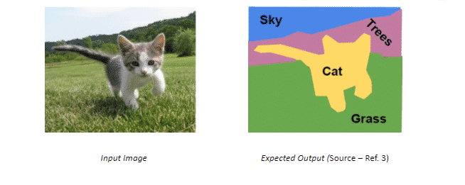
Also known as dense prediction, the goal of a semantic segmentation task is to label each pixel of the input image with the respective class representing a specific object/body. Segmentation is performed when the spatial information of a subject and how it interacts with it is important, like for an Autonomous vehicle.
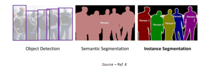
Also, one key thing to note is that this task is not interested in distinguishing multiple objects belonging to a certain class. For example, if you have two cars of different make and colour, they would still be given a common label of ‘Car’ and considered a single entity.
4. Instance Segmentation
Object Instance Segmentation takes semantic segmentation one step ahead in a sense that it aims towards distinguishing multiple objects from a single class. It can be considered as a Hybrid of Object Detection and Semantic Segmentation tasks.
Note – The scope of this article is limited to Semantic Segmentation using FCN only.
Various Applications of Semantic Segmentation
- Autonomous vehicles
- Medical image diagnostics
- Industrial Inspection
- Traffic Management, etc.
Now that we have a fair bit of understanding of what Semantic Segmentation is, and how it is different from the other Computer Vision tasks, we are ready to discuss in detail how Semantic Segmentation can be implemented.
Describing the Task at Hand –
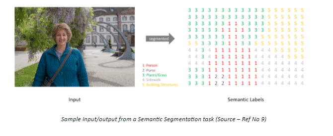
Simply put, given an input image of m x n x 3 shape (RGB), the model should be able to generate a m x n matrix filled with class labels as integers at the respective location.
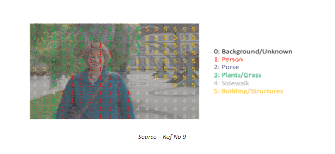
Implementing Semantic Segmentation –
- The naïve approach – Sliding Window
Segmentation can be achieved by using an Architecture similar to the Classification problem with a slight modification. Instead of one prediction on entire image, we can generate predictions for each pixel thus locating distinct classes in an image.
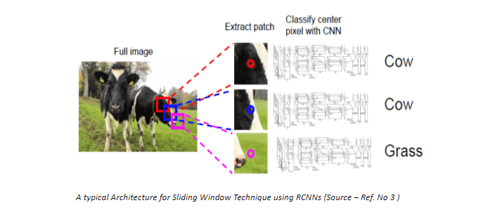
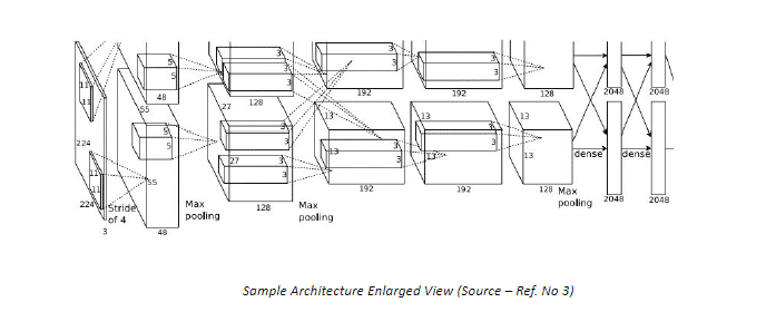
Although at a first glance this Architecture seems to be good enough for carrying out the Semantic Segmentation; however it has some major drawbacks -
- This approach involves prediction at individual pixel level, thus requiring a dense layer with enormous number of parameters that needs to be learned making it highly computationally expensive
- In addition, the use of dense layers as final output layers leads to a constraint on the dimension of the input image. A different architecture has to be defined for different input sizes
- No reusing of shared features takes place between overlapping patches, thus highly inefficient.
- Fully Convolutional Network
One way to counter the drawbacks of the previous Architecture is by stacking a number of Convolution Layers having similar padding to preserve dimension and output a final segmentation map. Meaning the model will learn the mapping from the input image to its corresponding segmentation map through the successive transformation of feature mappings.
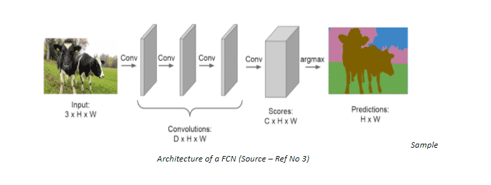
Seems good, but there is a major issue with this Architecture as well. We use the same padding in all the Convolution layers because we would want the output image to be of the same dimension as the input image. But this preservation of full-resolution becomes quite computationally expensive.
We could opt for a lesser number of layers, but that would damage the performance by a large margin.
We do not face this dilemma in a classification task because for that task we are only concerned about the presence of a single object of interest, losing the information about the location of the said object is harmless. Therefore, we can periodically downsample the images through pooling. However, this is not the case with Semantic Segmentation. If you want to segment a Highway image for training an autonomous vehicle, you would not want certain elements or vehicles to be cropped out from the final output that is fed to the machine.
- Fully Convolutional Network – with downsampling and upsampling inside the network!
A popular solution to the problem faced by the previous Architecture is by using Downsampling and Upsampling is a Fully Convolutional Network. In the first half of the model, we downsample the spatial resolution of the image developing complex feature mappings. With each convolution, we capture finer information of the image. At this stage, we obtain highly efficient discrimination between different classes; however, the information about the location is lost. To recover the location information, downsampling is followed by an upsampling procedure which takes multiple lower resolution images as input and gives a high-resolution segmentation map as output.
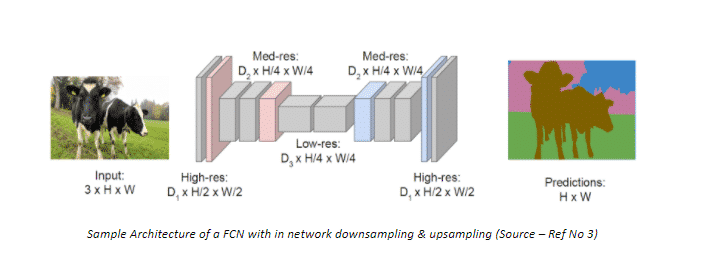
In the network presented above, it can be seen that the input image of resolution H x W is convoluted to H/2 x W/2 and finally to H/4 x W/4. At this stage we obtain mini heatmaps of different objects, each pixel highlighted to an intensity equivalent to the probability of occurrence of the object. As a next step, these mini heatmaps are upsampled and finally aggregated to obtain a High-resolution segmentation map, with each pixel classified into the highest probability class. Refer to the illustration below for a better understanding.
Keys Concepts –
- Convolution -
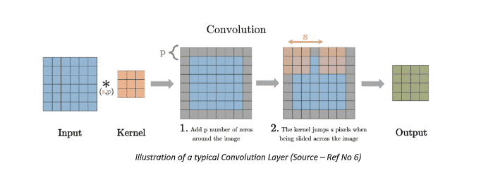
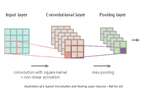
Convolution is the first layer which extracts features from an input image. Essentially, it is a matrix multiplication of the image matrix and a learnable filter matrix. The use of different filter matrices helps in extracting different features from the image. For example, filter A might capture all the vertical lines, while filter B captures all the Horizontal lines. The features get more and more complex as we go deeper in a convolution net, giving us a network which has the sequential holistic understanding of the image, very similar to how a Human would process any image.
- Pooling
Convolution is followed by the operation of Pooling, which is responsible for reducing the resolution of convoluted features even more, leading to reduced computational requirements. Also pooling leads to reduction of noise, and extraction of only the dominant features which are rotational and positional invariant.
Pooling can be carried out in two ways –
1. Max pooling – Returns the maximum value from the portion of the image
2. Average Pooling – Returns the average of all the values from the portion of image covered by the Kernel
- Unpooling – In network upsampling
After reducing the resolution by extracting convoluted features and pooling , for the case of Semantic Segmentation the next step is to upscale the low resolution back to the original resolution of the input image. Pooling converts a patch of values to a single value, whereas unpooling does the opposite, converts a single value into a patch of values.
Like Pooling, Unpooling can be carried out in different ways –
1. Nearest Neighbor
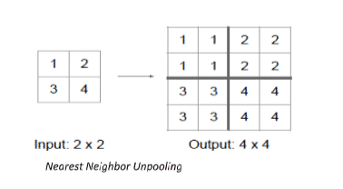
In Nearest neighbor approach, we pick a value and populate the surrounding cells with that value (no. of cells depending upon the increase in resolution), see value 1 being copied to every cell of the Top-Left 2x2 square.
2. Bed of Nails
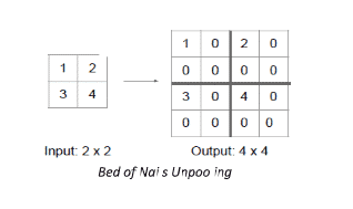
In this approach, instead of filling all the neighboring cells with a value, we fill the value at a predefined cell and fill the rest with 0, in the above example we fill the value in the top left cell of each 2x2 square.
3. Max Unpooling
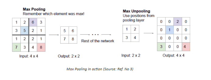
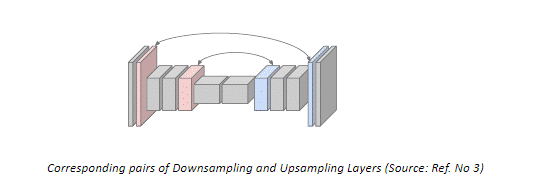
Max pooling is an improvement over “Bed of Nails” pooling, it utilises the symmetry present in a typical Downsampling-Upsampling Network, i.e for each Downsampling layer there exists a similar Upsampling layer as well. Rather than filling the value in a predefined cell, the value is filled in the cell having maximum value in the corresponding Downsampling layer.
- Transposed Convolution
Transposed Convolution or like some people incorrectly call it Deconvolution, can be seen as an opposite action to Convolution. Unlike convolution, a transposed convolution layer is used to upsample the reduced resolution feature back to its original resolution. A set of stride and padding values is learned to obtain the final output from the lower resolution features. The below illustration explains the procedure in a very easy to understand manner.

What makes transpose convolution better than other Upsampling techniques is that unlike previously described techniques (Nearest Neighbour, Bed of Nails, Max Unpooling), transpose convolution is a learnable upsampling making it highly efficient.
- Skip Connections
One major issue with in-network Downsampling in a FCN is that it reduces the resolution of the input by a large factor, thus during upsampling it becomes very difficult to reproduce the finer details even after using sophisticated techniques like Transpose Convolution. As a result we obtain a coarse output (refer the illustration below).
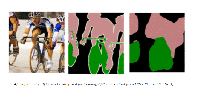
One-way to deal with this is by adding ‘skip connections’ in the Upsampling stage from earlier layers and summing the two feature maps. These skip connections provide enough information to later layers to generate accurate segmentation boundaries. This combination of fine and coarse layers leads to local predictions with nearly accurate global (spatial) structure.

The above illustrated network learns to combine coarse layer information with fine layer information. Layers are represented as grids with relative spatial coarseness, while the intermediate convolution layers of FCN are omitted for ease in understanding.
FCN-32s : Upsamples at stride 32, predictions back to pixels in a single step (Basic layer without any skip connections)
FCN-16s : Combines predictions from both the final layer and the pool4 layer with stride 16, finer details than FCN-32s.
FCN-8s : Adds predictions from pool3 at stride 8, providing even further precise boundaries.
Adding Skip connections can be considered as a Boosting method for a FCN, which tries to improve performance of layers by using predictions (feature maps) from previous layers.
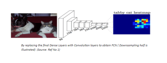
To summarize, this article started with an Introduction to Semantic Segmentation and compared it with the common Computer Vision tasks such as Classification, Object Detection. Followed up with the discussion on the three types of Networks to perform Segmentation, namely the Naïve sliding window network (classification task at the pixel level), FCNs ( replacing the final dense layers with convolution layers) and lastly FCNs with in-network Downsampling & Upsampling. To close off things, we lastly looked at key concepts concerning FCNs. Get your hands on this semantic segmentation tutorial today!
