Do you ever feel lost with Excel formulas and calculations? Or maybe you’re already comfortable with Excel, but want to learn advanced-level formulas?
This guide explains the formulas with examples, starting from the basics that everyone should know to more advanced levels that will help you solve complex calculations.
What are Excel Formulas?
Excel formulas are expressions that we use to perform calculations or manipulate data within a spreadsheet. They are made using predefined functions, mathematical operators, and cell references. Excel formulas are the backbone of data analysis. They help with tasks from basic operations like addition, multiplication, and subtraction to advanced statistical analysis.
Important Note:
- Formulas in Excel always start with an equal sign (=).
- If you make changes to the cell data that is referenced in the formula, Excel automatically re-calculates and updates the new result.
Why should you use Excel Formulas?
If you use Excel formulas you get several benefits, such as:
- Efficiency: Excel formulas can automate repetitive tasks and calculations, which saves time and improves productivity.
- Accuracy: When you use formulas, you’re less likely to make mistakes with numbers because Excel does the calculations for you, making sure everything is accurate.
- Automation: With the help of formulas, you can develop dynamic spreadsheets that change automatically as the data in linking cells and formulas change.
Excel Formulas List and Explanation with Examples
To help you understand better, we have categorized important and most used Excel functions in three levels:
- Basic Excel Formulas (Easy Calculations and Text Manipulation
- Intermediate (Logical Functions and Date/Time)
- Advanced (Lookups and Statistical Analysis)
Note: If you prefer learning through videos rather than text, you can learn these formulas through our video course. We offer a Free Excel Course, and after completing the course, you receive a certificate.
List of Basic Excel Formulas
1. SUM
The SUM function in Excel is used to add up the numbers in a range of cells. It’s one of the most popular functions and is quite easy to use.
Syntax: =SUM(number1, [number2], …)
For example, let’s say you have a list of certain numbers in cells D1 to D3:
=SUM(D1:D3)

To find the sum of these numbers, you can use the SUM function like this =SUM(D1:D3). This adds up all the numbers in selected cells, resulting in the sum of 30.
2. AVERAGE
The AVERAGE function in Excel calculates the average (mean) of a group of numbers.It adds up all the numbers in the specified range and then divides the sum by the count of those numbers.
Syntax: =AVERAGE(number1, [number2], …)
For example, Suppose you have exam grades in cells C1:C4. To find the average score, you can use the formula:
=AVERAGE(C1:C4)
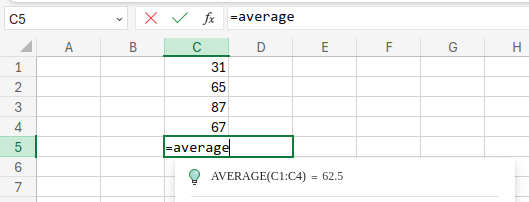
As you can see in the above image, this formula adds up all the numbers in the C1 to C4 range and then divides them by 4, returning the average value of 62.5.
3. COUNT and COUNTA
The COUNT function in Excel Counts cells with numbers. It specifically targets cells containing numeric data, including integers, decimals, and dates. It does not count texts.
Syntax: =COUNT(value1, [value2], …)
=COUNT(D1:D6)
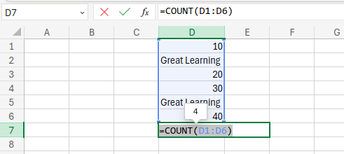
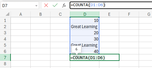
For counting cells with any kind of data (including text, numbers, and logical values), you should use the COUNTA function instead of COUNT.
Syntax: =COUNTA(value1, [value2], …)
=COUNTA(D1:D6)
4. MAX and MIN
MAX and MIN functions are used to find the largest and smallest values within a range of cells. The MAX function identifies the highest numerical value from a set of numbers. While the MIN function finds the lowest numerical value from a set of numbers.
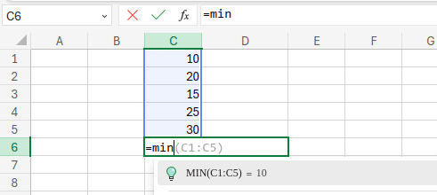
Suppose you have a list of certain numbers in cells C1 to C5:
Now, if you use the MAX function =MAX(C1:C5), it will return the maximum value from cells C1 to C5, which is 30 in this case.
=MAX(C1:C5)
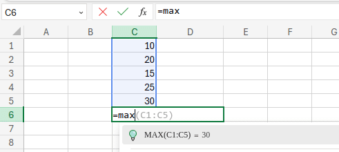
If you use the MIN function =MIN(C1:C5), it will return the minimum value from cells C1 to C5, which is 10 in this case.
=MIN(C1:C5)
5. CONCATENATE
The CONCATENATE function in Excel is used to combine multiple text strings or cell values into one single string. It is useful when you need to join text values from different cells together.
Syntax: =CONCATENATE(text1, [text2], …)
However, in newer versions of Excel, there’s an alternative method for concatenation using the ampersand (&) operator, which is more commonly used because it’s simpler and easier to understand. Let’s look at an example to understand easily.
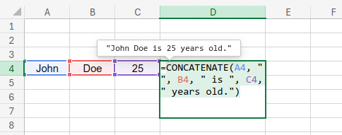
Suppose you have the following data in cells A4, B4, and C4:
A4= John, B4= Doe and C4= 25
To concatenate these values into one string, you can use either the CONCATENATE function or the ampersand (&) operator:
=CONCATENATE(A4, " ", B4, " is ", C4, " years old.")
Using the ampersand (&) operator: =A4 & ” ” & B4 & ” is ” & C4 & ” years old.”
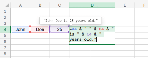
Both of these formulas will result in this concatenated string: John Doe is 25 years old.
6. LEN
The LEN function in Excel Counts the number of characters in text, including spaces, punctuation, and even letters and numbers. It also counts non-printable characters.
Syntax: =LEN(text)
Let’s look at an example to understand how to use the LEN function:
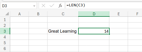
Suppose you have the text “Great Learning” in cell C3. To find out the length of this text string, you can use the LEN function like this:
=LEN(C3)
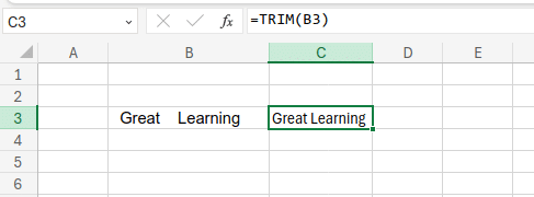
7. TRIM
The TRIM function is a text function that removes extra spaces from text strings for a cleaner, more consistent format. It removes all leading spaces (at the beginning of the text), trailing spaces (at the end), and extra spaces between words, leaving only a single space between each word.
Let’s say cell B3 contains the text ” Great Learning “. After applying the TRIM function, the result will be “Great Learning”.
=TRIM(text)
8. UPPER, LOWER and PROPER
UPPER, LOWER and PROPER are text formatting functions in Excel. The UPPER function converts all letters to uppercase, while the LOWER function converts all letters to lowercase.
The PROPER function converts text to proper case, where the first letter of each word is uppercase and all other letters are lowercase.
Example:
Imagine cell A1 contains the text “ThIs Is MiXeD CaSe”.
Using =UPPER(A1) will convert it to “THIS IS MIXED CASE”.
=UPPER(A1)
Using =LOWER(A1) will convert it to “this is mixed case”
=LOWER(A1)
Using =PROPER(A1) will convert it to “This Is Mixed Case”
=PROPER(A1)
Intermediate Level Excel Formulas
9. IF
The IF function is one of the most powerful and versatile functions in Excel. It allows you to perform conditional logic within your spreadsheets and return different values based on whether the test evaluates to TRUE or FALSE.
Syntax: =IF(logical_test, true_value, false_value)
Example:
Let’s say you have a list of exam scores in cell A2 and a passing grade of 70 in cell B2. You can use the following IF function to assign a pass/fail status in cell C2:
=IF(A2>=B2, "Pass", "Fail")
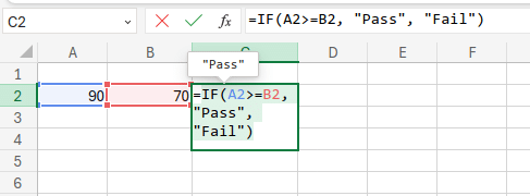
If the score in A2 is greater than or equal to the passing grade in B2 (TRUE), “Pass” is returned. If the score is lower than the passing grade (FALSE), “Fail” is returned.
10. VLOOKUP
The VLOOKUP is called Vertical Lookup. It is a function in Excel that is used to search for a value in the first column of a table or range, and then return a value in the same row from a specified column.
Syntax: =VLOOKUP(lookup_value, table_array, col_index_num, [range_lookup])
Example:
Imagine you have a table (A1:C10) containing product IDs (column A), product names (column B), and unit prices (column C). You want to find the unit price for a product with ID “ABC123” (stored in cell A6).
Here’s the formula you may use in cell
D3: =VLOOKUP(A6, A1:C10, 3, FALSE)
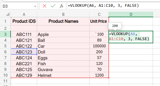
- A6: This is the cell containing the ID you want to look up (lookup_value).
- A1:C10 : This is the entire table where you want to search (table_array).
- 3: This specifies column C (unit prices), in which the data that you want to get is located (col_index_num).
- FALSE: This ensures an exact match for the ID (range_lookup). It’s an optional argument that determines how approximate matches should be handled. TRUE allows for inexact matches, while FALSE (default) requires an exact match.
11. COUNTIF
The COUNTIF function is like a friendly counter in Excel. It helps you count how many times something appears in a range of cells that meet a single condition.
Syntax: =COUNTIF(range, criteria)
Examples of Using COUNTIF:
- Counting cells with a specific text:
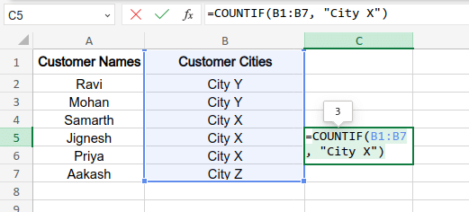
Suppose you have a customer list in cell range A2:A7, and their city name in B2 to B7. You want to count how many customers live in “City X”. You can use the formula:
=COUNTIF(B1:B7, "City X")
- Counting cells with numbers greater than a value:
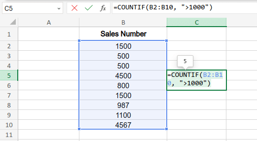
Let’s say you have sales data in cells B2:B10, and you want to know how many sales figures exceed $1000. You can use:
=COUNTIF(B2:B10, ">1000")
12. SUMIF
The SUMIF function in Excel is a powerful function that combines the functionality of SUM and IF. It helps you add up numbers in a range of cells based on a condition you specify.
Syntax: =SUMIF(criteria_range, criteria, sum_range)
Examples of Using SUMIF:
- Summing values based on text criteria:
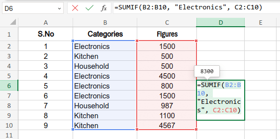
Suppose you have a sales data table with product categories in column B (B2:B10) and sales figures in column C (C2:C10). You want to find the total sales for the “Electronics” category. You can use the formula:
=SUMIF(B2:B10, "Electronics", C2:C10)
- Summing values based on a numerical condition:
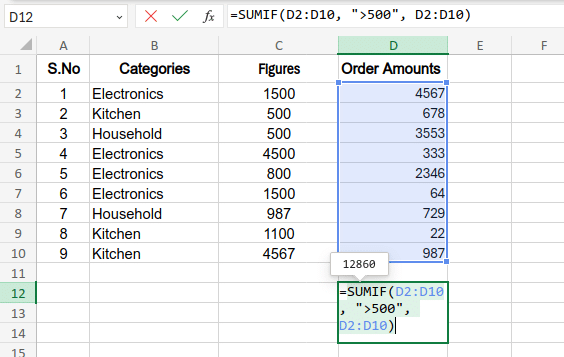
Let’s say you have order amounts in cells D2:D10 and want to calculate the total amount for orders exceeding $500. You can use:
=SUMIF(D2:D10, ">500", D2:D10)
13. TODAY and NOW
The TODAY function returns the current date on your system. Its syntax is: =TODAY()
While the NOW function Returns both the date and time as a combined value. The syntax of NOW is: =NOW()
For example, entering =TODAY() would display today’s date.
=TODAY()
And entering =NOW() would display Today’s date & time.
=NOW()
14. DAY, MONTH and YEAR
In Excel, DAY, MONTH, and YEAR functions are used for breaking down dates into smaller pieces. DAY tells you the day of the month, MONTH tells you the month number, and YEAR tells you the year.
Syntax:
- =DAY(date) Extracts the day number (1-31) from a date.
- =MONTH(date) Extracts the month number (1-12) from a date.
- =YEAR(date) Extracts the year as a four-digit number (YYYY) from a date.
Example:
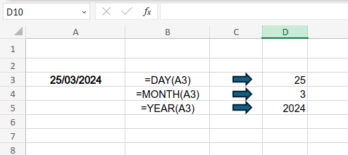
Let’s say you have a date in cell A3. You can use these functions to extract its components:
=DAY(A3)
=MONTH(A3)
=YEAR(A3)
Advanced Excel Formulas
15. INDEX & MATCH
The combination of INDEX and MATCH functions in Excel is very accurate and powerful for looking up values within a table. While VLOOKUP can only search for a value in the first column of a table and return a value from a specified column, INDEX and MATCH offer more flexibility. They can perform lookups based on multiple criteria.
1. MATCH Function:
The MATCH function is used to find a value’s position within a range. It returns the relative position of a specified value in a specified range of cells.
=MATCH(lookup_value, table_array, [match_type])
- lookup_value: This is the value you want to search for.
- table_array: This is the range of cells in which you want to search.
- [match_type]: This is an optional argument (0 or 1) specifying the search type:
- 0 for the exact match. It is by default and can be omitted.
- 1 for an approximate match. It is useful for sorted lists.
2. INDEX Function:
The INDEX function extracts a value from a specific location (row and column) within a range (table_array).
Syntax: =INDEX(table_array, row_num, [column_num])
How They Work Together:
- You can use the MATCH function to find the position of a lookup value within a range.
- You can use the INDEX function to retrieve the value from another range, using the position returned by MATCH.
For example, suppose you have a list of URLs in column A (A2:A10) and the category of those URLs in column B (B2:B10).
Now, there is a URL in C13, which you want to match with any URLs available in A2:A10 and retrieve the corresponding category available in B2:B10.
For this, you can combine the INDEX and MATCH functions and use the formula:
=INDEX(B2:B10, MATCH(C13, A2:A10,0))
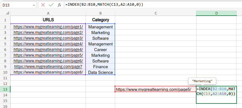
As you can see in the above image, the formula indexes the category “Marketing” from B2:B10 by matching the URLs in C13 with those in A2:A10.
16. COUNTIFS
The COUNTIFS function in Excel is used to count the number of cells that meet multiple criteria. It’s an extended version of the COUNTIF function, allowing you to specify multiple conditions for counting.
Syntax: =COUNTIFS(criteria_range1, criteria1, [criteria_range2, criteria2], …)
- criteria_range1, criteria_range2, etc., are the ranges of cells that you want to evaluate with specific criteria.
- criteria1, criteria2, etc., are the conditions or criteria that you want to apply to the corresponding ranges.
Example:
Let’s say, you have students’ names in column A (A2:A10), their Maths score in column B (B2:B10) and their English score in column C (C2:C10).
Now, you want to count the number of students who have scored above 80 in Maths and above 70 in English. For this, you can enter the following formula:
=COUNTIFS(B2:B10, ">80", C2:C10, ">70")
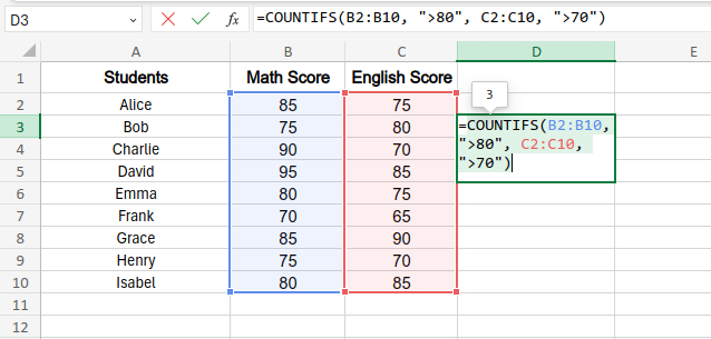
In this way, you can get the count of students who meet both criteria, which is 3 in this case.
17. SUMIFS
The SUMIFS function in Excel is an extension of the SUMIF function, used to sum the values in a range that meets multiple criteria.
Syntax: =SUMIFS(sum_range, criteria_range1, criteria1, [criteria_range2, criteria2], …)
For example, suppose you have product names in column A (A2:A10), regions where those products are available in column B (B2:B10) and product sales in column C (C2:C10).
Now, you want to find the total sales of product “ABC” in the “North” region. Here is how you can use the SUMIFS formula:
=SUMIFS(C2:C10, A2:A10, "ABC", B2:B10, "North")
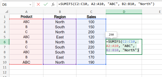
As you can see in this case, the formula does a sum based on multiple criteria and returns the value 290.
18. LEFT, RIGHT and MID
LEFT, RIGHT, and MID are like text scissors in Excel. They help you cut out specific parts of text from cells. They only work with text, so even if there are numbers or symbols, they treat them like letters.
- LEFT Function extracts a specified number of characters from the leftmost side of a text string. The syntax is =LEFT(text, num_chars)
- RIGHT Function extracts a specified number of characters from the rightmost side of a text string. The syntax is =RIGHT(text, num_chars)
- MID Function extracts a specific number of characters from a middle portion of a text string, starting at a specified position. The syntax is =MID(text, start_num, num_chars)
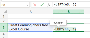
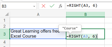
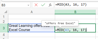
Lets understand these functions with the help of an example. Suppose cell A3 contains the text “Great Learning offers free Excel Course”.
If you use the formula =LEFT(A1, 5), it returns the first five characters.
=LEFT(A1, 5)
If you use =RIGHT(A3, 6), it returns the last 6 characters.
=RIGHT(A3, 6)
And if you use =MID(A3, 16, 17), it returns the specified middle portion.
=MID(A3, 16, 17)
19. REPLACE and SUBSTITUTE
- REPLACE
The REPLACE function in Excel is like a word surgery tool. It lets you remove a chunk of text from within a longer piece of text and replace it with something new. You tell it where to start removing text (start_num), how many characters to remove (num_chars), and what to put in their place (new_text).
Syntax: =REPLACE(text, start_num, num_chars, new_text)
Let’s say cell A3 contains the text “Hello World.” You want to replace “World” with “Universe” throughout the text. Here’s the formula:
=REPLACE(A3, 7, 5, "Universe")

This replaces the characters starting from the 7th position (W) for 5 characters with “Universe”, resulting in “Hello Universe”.
- SUBSTITUTE
The SUBSTITUTE function in Excel is like a find-and-replace tool for text. It lets you swap out all instances of a specific word or phrase with another word or phrase in a lengthy text. You only tell it what to look for and what to replace it with.
Syntax: =SUBSTITUTE(text, old_text, new_text)
Using the same text “Hello World” in cell A3, you can substitute “World” with “Universe” with:
=SUBSTITUTE(A3, "World", "Universe")

This formula will replace all instances of “World” with “Universe”, resulting in “Hello Universe”.
20. XLOOKUP
XLOOKUP is a new and powerful lookup function available in Excel versions newer than 2016. It combines the functionality of several older lookup functions (like VLOOKUP, HLOOKUP, and INDEX/MATCH)
Syntax: =XLOOKUP(lookup_value, lookup_array, return_array, [if_not_found], [match_mode], [search_mode])
It searches for a specific value (lookup_value) within a range (lookup_array) and returns a corresponding value from a different range (return_array).
For example, suppose you have a list of fruits in column A, their prices in column B, and the quantity in column E. Now, if you want to retrieve the quantity in column C using XLOOKUP, you can do it like this:
=XLOOKUP(A2, D:D, E:E)
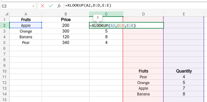
As shown above, the formula retrieves the quantity of fruits by searching for the fruit’s name in the lookup_array (column D).
Frequently Asked Questions
Q: Can Excel formulas handle large datasets?
A: Yes, Excel formulas are designed for working with big data. They can make calculations on thousands of rows at a time. However, when you have massive datasets, your computer’s speed and memory might affect performance. Consider using Excel’s built-in tools for large datasets or explore alternative solutions if necessary.
Q: I have a large dataset and need to find a specific value. What can I do?
A: Consider using VLOOKUP. It searches a table for a specific value in one column and returns data from a different column in the same row. (Note: VLOOKUP has limitations, use INDEX and MATCH for more complex scenarios.)
Q: My formula displays errors! What’s wrong?
A: There can be several reasons. Check for typos, incorrect cell references, or data inconsistencies. Excel’s =ISERROR function can also help identify error cells.
Q: Can formulas eliminate manual data analysis?
A: Excel formulas are powerful tools that reduce the need for manual calculations. They should, however, not replace data analysis completely. Instead of eliminating it, they make your manual analysis more efficient and accurate.
If you want to enhance Excel productivity and efficiency by reducing the need for manual mouse clicks, then you should know about the Most Used Excel Shortcuts.
Q: Are Excel formulas universal across all Excel versions?
A: The core Excel formulas you rely on remain consistent across most versions. However, newer versions often introduce additional functions and improved features to enhance your experience.
Q: Can I use formulas to format cells based on certain conditions?
A: Yes! Conditional formatting lets you apply formatting rules based on formula results. For example, highlight cells exceeding a value with a specific color.


