The Decision Tree Algorithm is one of the most widely used supervised learning techniques in machine learning. It is popular for its simplicity, interpretability, and effectiveness in handling both classification and regression problems.
Decision trees mimic human decision-making by splitting data into branches based on feature conditions, ultimately leading to a prediction.
What is a Decision Tree?
A decision tree is a tree-like structure where each internal node represents a feature (or attribute), each branch denotes a decision rule, and each leaf node represents an outcome or prediction. It breaks down complex decisions into a series of simpler choices, making it easy to interpret and understand.

Example: If you want to predict whether a person will buy a car, the decision tree may consider factors like income, age, and credit score. Based on these features, it will classify whether the person is likely to purchase the car or not.
Working of Decision Tree Algorithm

- Root Node Selection
- The process begins with the entire dataset.
- The best attribute (feature) to split on is selected based on a criterion like Gini impurity, Entropy, or Mean Squared Error (MSE) (for regression).
- Splitting the Dataset
- The selected feature divides the dataset into subsets.
- The split is chosen to maximize information gain (i.e., to reduce impurity as much as possible).
- Creating Branches & Nodes
- Each subset forms a branch leading to child nodes.
- The process continues recursively, selecting the best feature at each step to further split the data.
- Stopping Condition: Splitting stops when:
- A node becomes pure (i.e., all samples belong to the same class).
- A predefined depth limit is reached.
- The minimum number of samples per node is too small for further splitting.
- Prediction (Leaf Nodes)
- The final nodes (leaf nodes) hold the predicted class (for classification) or value (for regression).
- For new input data, the decision tree follows the path based on the feature conditions until it reaches a leaf node.
Example
Consider a simple classification task:
Dataset (Predict if a person buys a laptop based on Age & Salary)
| Age | Salary | Buys Laptop? |
| 25 | 50K | Yes |
| 40 | 30K | No |
| 30 | 70K | Yes |
| 50 | 90K | No |
A decision tree may look like:
- If Age < 35 → Yes
- If Age ≥ 35 → Check Salary
- If Salary < 60K → No
- If Salary ≥ 60K → Yes
Key Concepts:
- Gini Impurity: Measures how often a randomly chosen element would be incorrectly classified.
- Entropy: Measures disorder in data (higher entropy means more disorder, and we aim to reduce it).
- Information Gain: Determines which feature provides the most classification power.
- Pruning: Reduces overfitting by trimming unnecessary branches.
Learn how Alpha-Beta Pruning in AI optimizes decision-making in game theory by reducing unnecessary evaluations in the minimax algorithm.
Types of Decision Trees

- Classification Trees:
- These trees are used for categorical target variables where the output is discrete, such as "Yes/No" or "Spam/Not Spam."
- The tree is built by splitting the dataset based on feature values that maximize information gain.
- Example: Consider an email classification system. If an email contains words like "discount," "lottery," or "prize," the classification tree may decide whether the email is spam or not.
- Regression Trees:
- Regression trees are used when the target variable is continuous, such as predicting house prices or stock market values.
- Instead of classification, the tree predicts a numeric value based on feature splits.
- Example: Predicting the price of a house based on features like square footage, number of bedrooms, and location.
Advantages of Decision Trees

- Easy to Understand: The tree structure is intuitive and closely resembles human decision-making, making it easy to interpret.
- Handles Both Numerical and Categorical Data: Decision trees can work with different types of input data, unlike some machine learning algorithms that require numerical input only.
- Requires Minimal Data Preprocessing: No need for feature scaling, normalization, or dummy variable conversion.
- Feature Selection is Inbuilt: Decision trees inherently select the most important features, reducing dimensionality.
- Can Handle Missing Values: Some implementations of decision trees assign missing values to the most likely class or split them based on surrogate features.
Limitations of Decision Trees

- Overfitting: A deep decision tree with too many splits may fit the training data perfectly but fail to generalize well to unseen data.
- Unstable: Even small changes in the dataset can result in a significantly different tree structure, making decision trees sensitive to noise.
- Biased Towards Dominant Classes: If the dataset has an imbalance in class distribution, the decision tree may favor the dominant class, leading to skewed predictions.
- Computationally Expensive: Training large decision trees can be slow, especially when dealing with high-dimensional data.
Solution:
- Pruning: Reduces the complexity of the tree by removing less significant branches.
- Setting a Maximum Depth: Limits how deep the tree can grow to avoid overfitting.
- Ensemble Methods: Using techniques like Random Forest and Gradient Boosting improves performance by combining multiple trees.
Applications of Decision Trees

- Medical Diagnosis: Decision trees help in disease diagnosis by analyzing symptoms and patient history to suggest possible conditions.
- Customer Segmentation: Businesses use decision trees to group customers based on purchasing behavior, age, and demographics for targeted marketing campaigns.
- Fraud Detection: Banks and financial institutions use decision trees to identify fraudulent transactions by analyzing spending patterns and deviations from normal behavior.
- Recommendation Systems: E-commerce platforms suggest products to users based on browsing history and past purchases using decision trees.
- Credit Scoring: Loan approval systems evaluate applicants' creditworthiness by analyzing factors like income, credit score, and past loan history.
How to Implement a Decision Tree in Python
In this guide, you will learn how to implement a Decision Tree Classifier in Python using the Iris dataset. You will train the model, evaluate its accuracy, and visualize the decision tree step by step.
#Import Libraries
import matplotlib.pyplot as plt
from sklearn import tree
from sklearn.datasets import load_iris
from sklearn.tree import DecisionTreeClassifier
from sklearn.model_selection import train_test_split
from sklearn.metrics import accuracy_score

# Load Data
dataset = load_iris()
X, y = dataset.data, dataset.target
X_train, X_test, y_train, y_test = train_test_split(X, y, test_size=0.2, random_state=42)

# Train Decision Tree Model
dt_model = DecisionTreeClassifier(criterion='entropy', max_depth=3, random_state=42)
dt_model.fit(X_train, y_train)

# Make Predictions
y_pred = dt_model.predict(X_test)
accuracy = accuracy_score(y_test, y_pred)
print(f'Accuracy: {accuracy:.2f}')

# Visualize the Decision Tree
plt.figure(figsize=(10, 6))
tree.plot_tree(dt_model, filled=True, feature_names=dataset.feature_names, class_names=dataset.target_names)
plt.show()
Output: Accuracy: 1.00

Decision Tree vs. Other Machine Learning Algorithms
| Feature | Decision Tree | Random Forest | Logistic Regression |
| Interpretability | High | Moderate | Low |
| Overfitting | High | Low | Low |
| Computational Cost | Low | High | Low |
| Handles Non-Linear Data | Yes | Yes | No |
Conclusion
The Decision Tree Algorithm is a powerful yet simple machine learning model that is widely used in various domains. While it offers interpretability and ease of use, it also has limitations like overfitting and instability. However, techniques like pruning and ensemble methods can improve its performance.
If you are looking for an easy-to-implement and intuitive algorithm for classification and regression tasks, decision trees are a great starting point.
Learn how to build and optimize decision tree models with the free Decision Tree course. Gain hands-on experience in classification and regression techniques.
Frequently Asked Questions
1. What are the key parameters in a Decision Tree algorithm?
Decision trees have several important parameters, including max_depth (limits the depth of the tree to prevent overfitting), min_samples_split (minimum samples needed to split a node), and criterion (determines how the best split is selected, such as Gini impurity or entropy).
2. How does a Decision Tree handle missing values?
Decision Trees can handle missing data by assigning missing values to the most common class in classification problems or by estimating the missing values using surrogate splits in some implementations.
3. What is the difference between Decision Tree and Random Forest?
A Decision Tree is a single tree used for classification or regression, while Random Forest is an ensemble method that combines multiple decision trees to improve accuracy and reduce overfitting.
4. When should you not use a Decision Tree?
Decision Trees are not ideal for problems with high-dimensional data or cases where stability is crucial since they are prone to overfitting and are sensitive to small changes in data. In such cases, Random Forest or Gradient Boosting may be better alternatives.
5. Which industries use Decision Tree algorithms the most?
Decision Trees are widely used in finance (credit scoring, fraud detection), healthcare (medical diagnosis, treatment planning), marketing (customer segmentation, recommendation systems), and retail (demand forecasting, inventory management).


