Building a machine learning classification model involves several key steps, including data collection, exploration, preprocessing, and cleaning. After these steps, we apply classification techniques to generate predictions.
However, before finalizing a classifier model, we need to evaluate its performance. One essential tool for this evaluation is the Confusion Matrix, which measures classification accuracy and identifies errors.
In this article, we will explore the confusion matrix in detail and demonstrate its implementation in Python and R.
What is a Confusion Matrix?
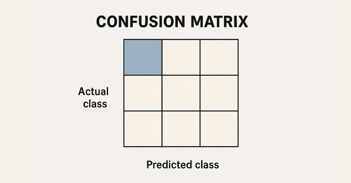
A confusion matrix is a table used to assess the performance of a classification model on a test dataset where the actual values are known. It is also referred to as an error matrix and provides insight into the types of errors the model makes. It categorizes predictions into four groups:

- True Positive (TP) – The actual value is positive, and the model correctly predicts it as positive.
- True Negative (TN) – The actual value is negative, and the model correctly predicts it as negative.
- False Positive (FP) – The actual value is negative, but the model predicts it as positive (Type I error).
- False Negative (FN) – The actual value is positive, but the model predicts it as negative (Type II error).
This structured table allows us to analyze model performance beyond simple accuracy calculations.
The Multiclass Classification concept is closely related to the confusion matrix, which helps assess the performance of models handling multiple categories.
Performance Metrics Derived from Confusion Matrix
The confusion matrix helps compute several performance metrics:

1. Accuracy
Formula: Accuracy = (TP + TN) / (TP + TN + FP + FN)
Accuracy measures how often the model makes correct predictions. However, in imbalanced datasets, high accuracy might be misleading.
2. Precision
Formula: Precision = TP / (TP + FP)
Precision measures how many predicted positive values are actually correct. It is crucial in applications like spam detection.
3. Recall (Sensitivity)
Formula: Recall = TP / (TP + FN)
Recall indicates how well the model identifies positive instances. A high recall means fewer false negatives.
4. F1-Score
Formula: F-measure = 2 * Recall * Precision / (Recall + Precision)
F1-Score balances precision and recall, making it useful when class distribution is uneven.
Understanding different Machine Learning Algorithms is essential, as the confusion matrix is commonly used to evaluate classification models.
Calculation of 2-class confusion matrix
Let us derive a confusion matrix and interpret the result using simple mathematics.
Let us consider the actual and predicted values of y as given below:
| Actual y | Y predicted | Predicted y with threshold 0.5 |
| 1 | 0.7 | 1 |
| 0 | 0.1 | 0 |
| 0 | 0.6 | 1 |
| 1 | 0.4 | 0 |
| 0 | 0.2 | 0 |
Now, if we make a confusion matrix from this, it would look like:
| N=5 | Predicted 1 | Predicted 0 |
| Actual: 1 | 1 (TP) | 1 (FN) |
| Actual: 0 | 1 (FP) | 2 (TN) |
This is our derived confusion matrix. Now we can also see all the four terms used in the above confusion matrix. Now we will find all the above-defined performance metrics from this confusion matrix.
1. Accuracy
Accuracy = (TP + TN) / (TP + TN + FP + FN)
So, Accuracy = (1+2) / (1+2+1+1)
= 3/5 which is 60%.
So, the accuracy from the above confusion matrix is 60%.
2. Precision
Precision = TP / (TP + FP)
= 1 / (1+1)
=1 / 2 which is 50%.
So, the precision is 50%.
3. Recall
Recall = TP / (TP + FN)
= 1 / (1+1)
= ½ which is 50%
So, the Recall is 50%.
4. F-measure
F-measure = 2 * Recall * Precision / (Recall + Precision)
= 2*0.5*0.5 / (0.5+0.5)
= 0.5
So, the F-measure is 50%.
Identifying Overfitting and Underfitting in Machine Learning is crucial when analyzing model performance, as a confusion matrix can highlight cases of misclassification.
Implementing Confusion Matrix in Python
Using scikit-learn, we can compute the confusion matrix and performance metrics:
import pandas as pd
import numpy as np
import matplotlib.pyplot as plt
import seaborn as sns
from sklearn.model_selection import train_test_split
from sklearn.linear_model import LogisticRegression
from sklearn.metrics import accuracy_score, confusion_matrix, classification_report

# Load dataset
df = pd.read_csv("bank.csv", delimiter=";")

# Data preprocessing
from sklearn.preprocessing import LabelEncoder
le = LabelEncoder()
df.job = le.fit_transform(df.job)
df.marital = le.fit_transform(df.marital)
df.y = le.fit_transform(df.y)

X = df.drop("y", axis=1)
y = df["y"]

# Train-Test Split
X_train, X_test, y_train, y_test = train_test_split(X, y, test_size=0.3, random_state=42)

# Model Training
model = LogisticRegression(max_iter=1000, random_state=42)
model.fit(X_train, y_train)
y_pred = model.predict(X_test)

# Evaluating Model
print("Accuracy:", accuracy_score(y_test, y_pred))
print("Confusion Matrix:\n", confusion_matrix(y_test, y_pred))
print("Classification Report:\n", classification_report(y_test, y_pred))
Output:

1. Accuracy: 48.67%
2. Confusion Matrix:
[79 72]
[82 67]
3. Classification Report
              precision    recall  f1-score   support

           0       0.49      0.52      0.51       151
           1       0.48      0.45      0.47       149

 accuracy                           0.49       300
macro avg       0.49      0.49      0.49       300
Implementing Confusion Matrix in R
In R, we use logistic regression for classification and confusion matrix computation:
library(dplyr)
library(ggplot2)
library(DataExplorer)

# Load dataset
df <- read.csv("adult.csv")

# Data Preprocessing
df$target <- ifelse(df$income == '>50K', 1, 0)
df$target <- as.factor(df$target)

# Train-Test Split
set.seed(1000)
index <- sample(nrow(df), 0.70 * nrow(df), replace=FALSE)
train <- df[index, ]
test <- df[-index, ]

# Logistic Regression Model
mod <- glm(target ~ ., data=train, family='binomial')
pred <- predict(mod, test, type='response')
pred_class <- ifelse(pred > 0.5, 1, 0)

# Confusion Matrix
table(Predicted=pred_class, Actual=test$target)
Conclusion
The confusion matrix is a fundamental tool for evaluating classification models. It provides insights into model accuracy, precision, recall, and F1-score. While accuracy is often the primary metric, recall and precision are crucial in various real-world applications, such as fraud detection and medical diagnoses.
By implementing confusion matrices in Python and R, we can better understand and optimize our machine learning models for improved performance.
Master Data Science and Machine Learning in Python with hands-on projects, real-world case studies, and expert-led lessons. Build job-ready skills in predictive modeling, feature engineering, and data analysis, and understand key evaluation techniques like the Confusion Matrix in Machine Learning, which helps assess model performance in classification tasks.
Frequently Asked Questions(FAQ’s)
1. What is the difference between a confusion matrix and a contingency table?
A confusion matrix is a special type of contingency table used for classification problems, where rows represent actual values and columns represent predicted values. A contingency table is a more general term used in statistics to display the frequency distribution of categorical variables.
2. Why is a confusion matrix important when accuracy is already given?
Accuracy alone can be misleading, especially in imbalanced datasets. A confusion matrix helps by showing False Positives (FP) and False Negatives (FN), which can be crucial in applications like medical diagnosis or fraud detection.
3. How does the confusion matrix change with imbalanced datasets?
In imbalanced datasets, the model tends to favor the majority class, leading to a misleadingly high accuracy. A confusion matrix reveals whether the model is simply predicting the dominant class, making metrics like Precision, Recall, and F1-score more important.
4. Can we use a confusion matrix for multi-class classification?
Yes, a confusion matrix can handle multi-class classification. Instead of a 2×2 matrix, it becomes an N×N matrix, where N is the number of classes. Each cell represents the count of true vs. predicted values for a particular class.
5. How can I normalize a confusion matrix for better interpretation?
A raw confusion matrix shows absolute counts, which can be hard to interpret when class distributions vary. You can normalize it using:
cm_normalized = cm.astype('float') / cm.sum(axis=1)[:, np.newaxis]
This converts the confusion matrix values into percentages, making it easier to compare across classes.


