Computer Vision Using PyTorch with Example

Computer vision is one of the most exciting and rapidly evolving fields in artificial intelligence (AI). It enables machines to interpret and understand the visual world. With the rise of deep learning, frameworks like PyTorch have made it easier than ever for developers and researchers to build and train advanced computer vision models. 

In this guide, we’ll explore computer vision using PyTorch with a practical example of implementing a Convolutional Neural Network (CNN).

What is Computer Vision?

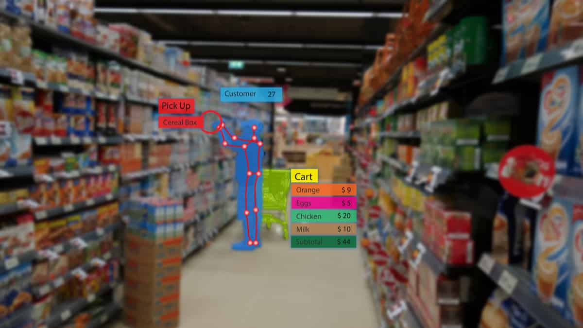
Computer vision is the field of AI that enables machines to process and interpret visual information from the world, such as images or videos. Tasks in computer vision include image classification, object detection, face recognition, and image segmentation.

Why Use PyTorch for Computer Vision?

PyTorch is an ideal framework for computer vision, offering powerful features that facilitate flexibility, experimentation, and widespread adoption among AI researchers.

• Flexibility: Versatile environment for building deep learning models.
• Easy-to-use Features: Simplifies model development and experimentation.
• Dynamic Computation Graphs: Enables rapid experimentation with adjustable models.

In computer vision, PyTorch provides quite a few predefined and already-implemented infrastructures, such as those related to image data: GPU-based training of models, and neural network building with least effort imaginable.

Getting Started with PyTorch for Computer Vision

Before we dive into building a computer vision model, let’s ensure that PyTorch is properly installed on your system.

Installing PyTorch

To install PyTorch along with torchvision (which contains essential utilities for working with image data), use the following command:

pip install torch torchvision

Once installed, you can check if PyTorch is correctly installed by running:

import torch
print(torch.__version__)

Understanding Tensors in PyTorch

At the core of PyTorch is the tensor, which is a multi-dimensional array. In the context of computer vision, images are represented as tensors. For instance:

• A grayscale image is represented as a 2D tensor (height x width).

• A color image (RGB) is represented as a 3D tensor (height x width x 3), where 3 corresponds to the three color channels: Red, Green, and Blue.

PyTorch provides a convenient way to manipulate and process tensors, allowing us to perform tasks like element-wise operations, reshaping, and matrix multiplication.

Steps to Build a Simple CNN for Image Classification

In this section, we’ll build a simple Convolutional Neural Network (CNN) in PyTorch to classify handwritten digits from the MNIST dataset, a popular dataset for testing machine learning algorithms.

Step 1: Load and Preprocess the Data

We’ll start by loading the MNIST dataset and applying some necessary transformations to prepare it for training.

import torch
import torch.nn as nn
import torch.optim as optim
import torchvision
import torchvision.transforms as transforms

# Define the transformations
transform = transforms.Compose([
    transforms.ToTensor(),  # Convert images to tensors
    transforms.Normalize((0.5,), (0.5,))  # Normalize images
])

# Download the MNIST dataset
trainset = torchvision.datasets.MNIST(root='./data', train=True, download=True, transform=transform)
testset = torchvision.datasets.MNIST(root='./data', train=False, download=True, transform=transform)

# Create data loaders to load the data in batches
trainloader = torch.utils.data.DataLoader(trainset, batch_size=64, shuffle=True)
testloader = torch.utils.data.DataLoader(testset, batch_size=64, shuffle=False)

Here, we:

• Use ToTensor() to convert images into PyTorch tensors.
• Normalize the images so that they have a mean of 0.5 and a standard deviation of 0.5.
• Download the MNIST dataset and prepare the data loaders to handle the data in batches.

Step 2: Define the CNN Architecture

Next, we’ll define a simple CNN with one convolutional layer, one pooling layer, and one fully connected layer.

class SimpleCNN(nn.Module):
    def __init__(self):
        super(SimpleCNN, self).__init__()
        
        # Define the layers
        self.conv1 = nn.Conv2d(1, 32, kernel_size=3)  # Conv layer: 1 input channel (grayscale), 32 output channels
        self.pool = nn.MaxPool2d(2, 2)  # Max pooling layer
        self.fc1 = nn.Linear(32 * 6 * 6, 10)  # Fully connected layer

    def forward(self, x):
        x = self.pool(torch.relu(self.conv1(x)))  # Apply conv, ReLU activation, and pooling
        x = x.view(-1, 32 * 6 * 6)  # Flatten the tensor for the fully connected layer
        x = self.fc1(x)  # Apply the fully connected layer
        return x

This CNN:

• conv1: A convolutional layer with 1 input channel and 32 output channels, using a kernel size of 3.
• pool: A max-pooling layer with a 2×2 kernel to downsample the feature maps.
• fc1: A fully connected layer with 10 output units (one for each digit in the MNIST dataset).

Step 3: Initialize the Model, Loss Function, and Optimizer

We will now initialize the model, specify a loss function, and choose an optimizer.

model = SimpleCNN()

# Loss function: CrossEntropyLoss is used for multi-class classification
criterion = nn.CrossEntropyLoss()

# Optimizer: Stochastic Gradient Descent (SGD)
optimizer = optim.SGD(model.parameters(), lr=0.001, momentum=0.9)

Step 4: Train the Model

Now we’ll train the model by iterating through the dataset for a few epochs. For each batch of data:

1. Perform a forward pass to get predictions.
2. Calculate the loss.
3. Perform a backward pass to compute gradients.
4. Update the weights with the optimizer.

for epoch in range(5):  # Train for 5 epochs
    running_loss = 0.0
    for i, data in enumerate(trainloader, 0):
        inputs, labels = data
        
        # Zero the gradients
        optimizer.zero_grad()
        
        # Forward pass: get predictions
        outputs = model(inputs)
        
        # Calculate the loss
        loss = criterion(outputs, labels)
        
        # Backward pass: compute gradients
        loss.backward()
        
        # Update the weights
        optimizer.step()
        
        running_loss += loss.item()

    print(f"Epoch {epoch+1}, Loss: {running_loss/len(trainloader)}")

Step 5: Evaluate the Model

After training, we’ll evaluate the model on the test dataset to measure its accuracy.

# Evaluate the model
correct = 0
total = 0
with torch.no_grad():  # No need to compute gradients during evaluation
    for data in testloader:
        images, labels = data
        outputs = model(images)
        _, predicted = torch.max(outputs, 1)  # Get predicted labels
        total += labels.size(0)
        correct += (predicted == labels).sum().item()

print(f"Accuracy on the test set: {100 * correct / total}%")

Step 6: Save the Model

Once you’ve trained the model, you can save it for later use.

# Save the trained model
torch.save(model.state_dict(), 'simple_cnn.pth')

Conclusion

In this guide, we’ve walked through the process of implementing computer vision using PyTorch. We covered the following:

• Loading and preprocessing the MNIST dataset.
• Defining a simple CNN architecture.
• Training the model using PyTorch.
• Evaluating the model on a test dataset.
• Saving the model for later use.

By following these steps, you can easily implement your own computer vision models using PyTorch for tasks like image classification, object detection, and more. With practice and experimentation, you’ll be able to enhance and optimize these models for real-world applications.

If you’re just getting started, explore our free Computer Vision Essentials course to gain hands-on experience with Python and TensorFlow.

For those looking to take their AI skills to the next level, check out our comprehensive AI & Machine Learning program, featuring advanced topics like computer vision, deep learning, and real-world projects.

Frequently Asked Questions

1. What is data augmentation, and why is it important in computer vision?

Data augmentation artificially expands the dataset by applying random transformations like rotation, flipping, and image scaling. This helps prevent overfitting and improves model generalization by introducing more diverse training examples.

To learn various data augmentation techniques and their impact on computer vision models, check out our article on Data Augmentation.

2. What is the role of ReLU activation in CNNs?

ReLU (Rectified Linear Unit) introduces non-linearity in the network by outputting zero for negative values and leaving positive values unchanged. It helps CNNs learn complex patterns and accelerates convergence during training by mitigating the vanishing gradient problem.

3. How can I optimize the performance of my CNN model?

To optimize performance, try using advanced techniques such as dropout, batch normalization, or experimenting with more complex architectures like ResNet. You can also fine-tune hyperparameters like learning rate, batch size, and optimizer type to achieve better accuracy.