Machine Learning problems deal with a great deal of data and depend heavily on the algorithms that are used to train the model. There are various approaches and algorithms to train a machine learning model based on the problem at hand. Supervised and unsupervised learning are the two most prominent of these approaches. An important real-life problem of marketing a product or service to a specific target audience can be easily resolved with the help of a form of unsupervised learning known as Clustering. This article will explain clustering algorithms along with real-life problems and examples. Let us start with understanding what clustering is.
What are Clusters?
The word cluster is derived from an old English word, ‘clyster, ‘ meaning a bunch. A cluster is a group of similar things or people positioned or occurring closely together. Usually, all points in a cluster depict similar characteristics; therefore, machine learning could be used to identify traits and segregate these clusters. This makes the basis of many applications of machine learning that solve data problems across industries.
What is Clustering?
As the name suggests, clustering involves dividing data points into multiple clusters of similar values. In other words, the objective of clustering is to segregate groups with similar traits and bundle them together into different clusters. It is ideally the implementation of human cognitive capability in machines enabling them to recognize different objects and differentiate between them based on their natural properties. Unlike humans, it is very difficult for a machine to identify an apple or an orange unless properly trained on a huge relevant dataset. Unsupervised learning algorithms achieve this training, specifically clustering.
Simply put, clusters are the collection of data points that have similar values or attributes and clustering algorithms are the methods to group similar data points into different clusters based on their values or attributes.
For example, the data points clustered together can be considered as one group or cluster. Hence the diagram below has two clusters (differentiated by color for representation).
Why Clustering?
When you are working with large datasets, an efficient way to analyze them is to first divide the data into logical groupings, aka clusters. This way, you could extract value from a large set of unstructured data. It helps you to glance through the data to pull out some patterns or structures before going deeper into analyzing the data for specific findings.
Organizing data into clusters helps identify the data’s underlying structure and finds applications across industries. For example, clustering could be used to classify diseases in the field of medical science and can also be used in customer classification in marketing research.
In some applications, data partitioning is the final goal. On the other hand, clustering is also a prerequisite to preparing for other artificial intelligence or machine learning problems. It is an efficient technique for knowledge discovery in data in the form of recurring patterns, underlying rules, and more. Try to learn more about clustering in this free course: Customer Segmentation using Clustering
Types of Clustering Methods/ Algorithms
Given the subjective nature of the clustering tasks, there are various algorithms that suit different types of clustering problems. Each problem has a different set of rules that define similarity among two data points, hence it calls for an algorithm that best fits the objective of clustering. Today, there are more than a hundred known machine learning algorithms for clustering.
A few Types of Clustering Algorithms
- Connectivity Models
As the name indicates, connectivity models tend to classify data points based on their closeness of data points. It is based on the notion that the data points closer to each other depict more similar characteristics compared to those placed farther away. The algorithm supports an extensive hierarchy of clusters that might merge with each other at certain points. It is not limited to a single partitioning of the dataset.
The choice of distance function is subjective and may vary with each clustering application. There are also two different approaches to addressing a clustering problem with connectivity models. First is where all data points are classified into separate clusters and then aggregated as the distance decreases. The second approach is where the whole dataset is classified as one cluster and then partitioned into multiple clusters as the distance increases. Even though the model is easily interpretable, it lacks the scalability to process bigger datasets.
- Distribution Models
Distribution models are based on the probability of all data points in a cluster belonging to the same distribution, i.e., Normal distribution or Gaussian distribution. The slight drawback is that the model is highly prone to suffering from overfitting. A well-known example of this model is the expectation-maximization algorithm.
- Density Models
These models search the data space for varied densities of data points and isolate the different density regions. It then assigns the data points within the same region as clusters. DBSCAN and OPTICS are the two most common examples of density models.
- Centroid Models
Centroid models are iterative clustering algorithms where similarity between data points is derived based on their closeness to the cluster’s centroid. The centroid (center of the cluster) is formed to ensure that the distance of the data points is minimal from the center. The solution for such clustering problems is usually approximated over multiple trials. An example of centroid models is the K-means algorithm.
Common Clustering Algorithms
K-Means Clustering
K-Means is by far the most popular clustering algorithm, given that it is very easy to understand and apply to a wide range of data science and machine learning problems. Here’s how you can apply the K-Means algorithm to your clustering problem.
The first step is randomly selecting a number of clusters, each of which is represented by a variable ‘k’. Next, each cluster is assigned a centroid, i.e., the center of that particular cluster. It is important to define the centroids as far off from each other as possible to reduce variation. After all the centroids are defined, each data point is assigned to the cluster whose centroid is at the closest distance.
Once all data points are assigned to respective clusters, the centroid is again assigned for each cluster. Once again, all data points are rearranged in specific clusters based on their distance from the newly defined centroids. This process is repeated until the centroids stop moving from their positions.
K-Means algorithm works wonders in grouping new data. Some of the practical applications of this algorithm are in sensor measurements, audio detection, and image segmentation.
Let us have a look at the R implementation of K Means Clustering.
K Means clustering with ‘R’
- Having a glance at the first few records of the dataset using the head() function
head(iris)
##   Sepal.Length Sepal.Width Petal.Length Petal.Width Species
## 1          5.1         3.5          1.4         0.2  setosa
## 2          4.9         3.0          1.4         0.2  setosa
## 3          4.7         3.2          1.3         0.2  setosa
## 4          4.6         3.1          1.5         0.2  setosa
## 5          5.0         3.6          1.4         0.2  setosa
## 6          5.4         3.9          1.7         0.4  setosa
- Removing the categorical column ‘Species’ because k-means can be applied only on numerical columns
iris.new<- iris[,c(1,2,3,4)]

head(iris.new)
##   Sepal.Length Sepal.Width Petal.Length Petal.Width
## 1          5.1         3.5          1.4         0.2
## 2          4.9         3.0          1.4         0.2
## 3          4.7         3.2          1.3         0.2
## 4          4.6         3.1          1.5         0.2
## 5          5.0         3.6          1.4         0.2
## 6          5.4         3.9          1.7         0.4
- Making a scree-plot to identify the ideal number of clusters
totWss=rep(0,5)
for(k in 1:5){
  set.seed(100)
  clust=kmeans(x=iris.new, centers=k, nstart=5)
  totWss[k]=clust$tot.withinss
}
plot(c(1:5), totWss, type="b", xlab="Number of Clusters",
     ylab="sum of 'Within groups sum of squares'")
- Visualizing the clustering
library(cluster)
library(fpc)

## Warning: package 'fpc' was built under R version 3.6.2

clus <- kmeans(iris.new, centers=3)

plotcluster(iris.new, clus$cluster)
clusplot(iris.new, clus$cluster, color=TRUE,shade = T)
- Adding the clusters to the original dataset
iris.new<-cbind(iris.new,cluster=clus$cluster)

head(iris.new)
##   Sepal.Length Sepal.Width Petal.Length Petal.Width cluster
## 1          5.1         3.5          1.4         0.2       1
## 2          4.9         3.0          1.4         0.2       1
## 3          4.7         3.2          1.3         0.2       1
## 4          4.6         3.1          1.5         0.2       1
## 5          5.0         3.6          1.4         0.2       1
## 6          5.4         3.9          1.7         0.4       1
Density-Based Spatial Clustering of Applications With Noise (DBSCAN)
DBSCAN is the most common density-based clustering algorithm and is widely used. The algorithm picks an arbitrary starting point, and the neighborhood to this point is extracted using a distance epsilon ‘ε’. All the points that are within the distance epsilon are the neighborhood points. If these points are sufficient in number, then the clustering process starts, and we get our first cluster. If there are not enough neighboring data points, then the first point is labeled noise.
For each point in this first cluster, the neighboring data points (the one which is within the epsilon distance with the respective point) are also added to the same cluster. The process is repeated for each point in the cluster until there are no more data points that can be added.
Once we are done with the current cluster, an unvisited point is taken as the first data point of the next cluster, and all neighboring points are classified into this cluster. This process is repeated until all points are marked ‘visited’.
DBSCAN has some advantages as compared to other clustering algorithms:
- It does not require a pre-set number of clusters
- Identifies outliers as noise
- Ability to find arbitrarily shaped and sized clusters easily
Implementing DBSCAN with Python
from sklearn import datasets
import numpy as np
import pandas as pd
import matplotlib.pyplot as plt
from sklearn.cluster import DBSCAN

iris = datasets.load_iris()
x = iris.data[:, :4]  # we only take the first two features.
DBSC = DBSCAN()
cluster_D = DBSC.fit_predict(x)
print(cluster_D)
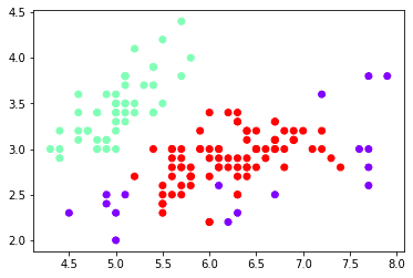
plt.scatter(x[:,0],x[:,1],c=cluster_D,cmap='rainbow')
[ 0 0 0 0 0 0 0 0 0 0 0 0 0 0 0 0 0 0 0 0 0 0 0 0 0 0 0 0 0 0 0 0 0 0 0 0 0 0 0 0 0 -1 0 0 0 0 0 0 0 0 1 1 1 1 1 1 1 -1 1 1 -1 1 1 1 1 1 1 1 -1 1 1 1 1 1 1 1 1 1 1 1 1 1 1 1 1 1 1 -1 1 1 1 1 1 -1 1 1 1 1 -1 1 1 1 1 1 1 -1 -1 1 -1 -1 1 1 1 1 1 1 1 -1 -1 1 1 1 -1 1 1 1 1 1 1 1 1 -1 1 1 -1 -1 1 1 1 1 1 1 1 1 1 1 1 1 1 1]
<matplotlib.collections.PathCollection at 0x7f38b0c48160>
Hierarchical Clustering
Hierarchical Clustering is categorized into divisive and agglomerative clustering. Basically, these algorithms have clusters sorted in an order based on the hierarchy in data similarity observations.
Divisive Clustering, or the top-down approach, groups all the data points in a single cluster. Then it divides it into two clusters with the least similarity to each other. The process is repeated, and clusters are divided until there is no more scope for doing so.
Agglomerative Clustering, or the bottom-up approach, assigns each data point as a cluster and aggregates the most similar clusters. This essentially means bringing similar data together into a cluster.
Out of the two approaches, Divisive Clustering is more accurate. But then, it again depends on the type of problem and the nature of the available dataset to decide which approach to apply to a specific clustering problem in Machine Learning.
Implementing Hierarchical Clustering with Python
#Import libraries
from sklearn import datasets
import numpy as np
import pandas as pd
import matplotlib.pyplot as plt
from sklearn.cluster import AgglomerativeClustering

#import the dataset
iris = datasets.load_iris()
x = iris.data[:, :4]  # we only take the first two features.
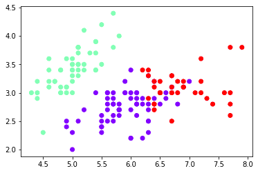
hier_clustering = AgglomerativeClustering(3)
clusters_h = hier_clustering.fit_predict(x)
print(clusters_h )
plt.scatter(x[:,0],x[:,1],c=clusters_h ,cmap='rainbow')
[1 1 1 1 1 1 1 1 1 1 1 1 1 1 1 1 1 1 1 1 1 1 1 1 1 1 1 1 1 1 1 1 1 1 1 1 1 1 1 1 1 1 1 1 1 1 1 1 1 1 0 0 0 0 0 0 0 0 0 0 0 0 0 0 0 0 0 0 0 0 0 0 0 0 0 0 0 2 0 0 0 0 0 0 0 0 0 0 0 0 0 0 0 0 0 0 0 0 0 0 2 0 2 2 2 2 0 2 2 2 2 2 2 0 0 2 2 2 2 0 2 0 2 0 2 2 0 0 2 2 2 2 2 0 0 2 2 2 0 2 2 2 0 2 2 2 0 2 2 0]
<matplotlib.collections.PathCollection at 0x7f38b0bcbb00>
Applications of Clustering
Clustering has varied applications across industries and is an effective solution to a plethora of machine learning problems.
- It is used in market research to characterize and discover a relevant customer bases and audiences.
- Classifying different species of plants and animals with the help of image recognition techniques
- It helps in deriving plant and animal taxonomies and classifies genes with similar functionalities to gain insight into structures inherent to populations.
- It is applicable in city planning to identify groups of houses and other facilities according to their type, value, and geographic coordinates.
- It also identifies areas of similar land use and classifies them as agricultural, commercial, industrial, residential, etc.
- Classifies documents on the web for information discovery
- Applies well as a data mining function to gain insights into data distribution and observe characteristics of different clusters
- Identifies credit and insurance frauds when used in outlier detection applications
- Helpful in identifying high-risk zones by studying earthquake-affected areas (applicable for other natural hazards too)
- A simple application could be in libraries to cluster books based on the topics, genre, and other characteristics
- An important application is into identifying cancer cells by classifying them against healthy cells
- Search engines provide search results based on the nearest similar object to a search query using clustering techniques
- Wireless networks use various clustering algorithms to improve energy consumption and optimise data transmission
- Hashtags on social media also use clustering techniques to classify all posts with the same hashtag under one stream
In this article, we discussed different clustering algorithms in Machine Learning. While there is so much more to unsupervised learning and machine learning as a whole, this article specifically draws attention to clustering algorithms in Machine Learning and their applications. If you want to learn more about machine learning concepts, head to our blog. Also, if you wish to pursue a career in Machine Learning, then upskill with Great Learning’s PG program in Machine Learning.


