Characteristic Equation for Data Science and its Applications

Data science is often viewed as a blend of programming, statistics, and domain expertise, but beneath the surface, linear algebra forms its backbone. 

The characteristic equation, a fundamental concept in matrix theory, plays a pivotal role in various techniques like eigenvalue decomposition, stability analysis, and principal component analysis (PCA).

This article will unravel its importance and showcase real-world applications where it enhances data-driven decision-making.

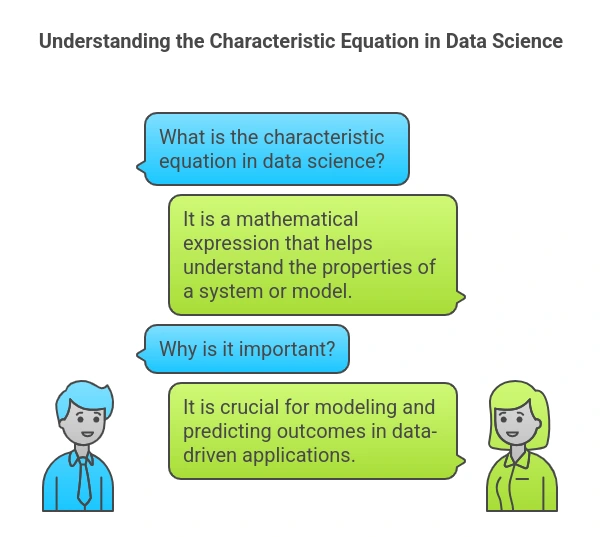
Definition and Mathematical Formulation

The characteristic equation is a key mathematical tool used in linear algebra to determine the eigenvalues of a square matrix. It is essential for understanding transformations, stability, and dimensionality reduction techniques used in data science.

For a given n×nn \times nn×n square matrix AAA, the characteristic equation is defined as:

∣A−λI∣=0|A - \lambda I| = 0∣A−λI∣=0

Where:

• AAA is the given matrix,
• λ\lambdaλ represents the eigenvalues of AAA,
• III is the identity matrix of the same size as AAA,
• ∣A−λI∣|A – \lambda I|∣A−λI∣ denotes the determinant of the matrix (A−λI)(A – \lambda I)(A−λI).

By solving this determinant equation, we obtain a polynomial (known as the characteristic polynomial) whose roots correspond to the eigenvalues of AAA. 

These eigenvalues provide crucial insights into the matrix’s properties, including stability, transformation effects, and system behavior in various applications.

Explanation of Eigenvalues and Eigenvectors

Eigenvalues and eigenvectors are fundamental concepts in linear algebra and are widely used in data science, machine learning, and other computational fields.

• An eigenvalue λ\lambdaλ of a matrix AAA satisfies the equation:
  Av=λvA v = \lambda vAv=λv
  where vvv is a nonzero vector, called an eigenvector.
• This equation implies that when matrix AAA acts on the vector vvv, it scales the vector by a factor of λ\lambdaλ, rather than changing its direction.

Geometric Interpretation

• Eigenvectors represent principal directions in which a linear transformation occurs.
• Eigenvalues indicate how much the vector is stretched or compressed along that direction.
• If λ>1\lambda > 1λ>1, the vector is stretched.
• If 0<λ<10 < \lambda < 10<λ<1, the vector is shrunk.
• If λ=0\lambda = 0λ=0, the transformation collapses the vector into the origin.
• If λ\lambdaλ is negative, the vector is flipped.

Example: Finding Eigenvalues and Eigenvectors

Consider the matrix:

A=[4123]A = \begin{bmatrix} 4 & 1 \\ 2 & 3 \end{bmatrix}A=[42​13​]

To find its eigenvalues, we solve:

∣4−λ123−λ∣=0\begin{vmatrix} 4 - \lambda & 1 \\ 2 & 3 - \lambda \end{vmatrix} = 0​4−λ2​13−λ​​=0

Expanding the determinant:

(4−λ)(3−λ)−(1)(2)=0(4 - \lambda)(3 - \lambda) - (1)(2) = 0(4−λ)(3−λ)−(1)(2)=0 λ2−7λ+10=0\lambda^2 - 7\lambda + 10 = 0λ2−7λ+10=0

Solving for λ\lambdaλ:

λ=7±49−402=7±32\lambda = \frac{7 \pm \sqrt{49 - 40}}{2} = \frac{7 \pm 3}{2}λ=27±49−40​​=27±3​ λ1=5,λ2=2\lambda_1 = 5, \quad \lambda_2 = 2λ1​=5,λ2​=2

Thus, the eigenvalues of AAA are 5 and 2. These values indicate how vectors along specific directions are scaled when transformed by AAA.

To find the corresponding eigenvectors, we solve:

(A−λI)v=0(A - \lambda I)v = 0(A−λI)v=0

For λ=5\lambda = 5λ=5:

[−112−2][xy]=0\begin{bmatrix} -1 & 1 \\ 2 & -2 \end{bmatrix} \begin{bmatrix} x \\ y \end{bmatrix} = 0[−12​1−2​][xy​]=0

Solving, we get:

x=yx = yx=y

Thus, one eigenvector is:

v1=[11]v_1 = \begin{bmatrix} 1 \\ 1 \end{bmatrix}v1​=[11​]

For λ=2\lambda = 2λ=2:

[2121][xy]=0\begin{bmatrix} 2 & 1 \\ 2 & 1 \end{bmatrix} \begin{bmatrix} x \\ y \end{bmatrix} = 0[22​11​][xy​]=0

Solving, we get:

x=−0.5yx = -0.5yx=−0.5y

Thus, another eigenvector is:

v2=[−12]v_2 = \begin{bmatrix} -1 \\ 2 \end{bmatrix}v2​=[−12​]

These eigenvectors correspond to the directions in which the matrix transformation scales vectors.

Basic Properties and Interpretations

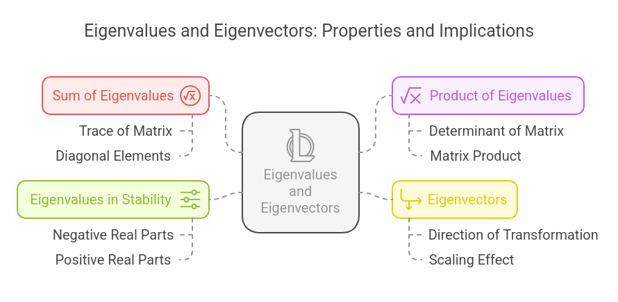
1. Sum of Eigenvalues = Trace of Matrix

The sum of the eigenvalues of a matrix equals the sum of its diagonal elements (trace of AAA).

∑λi=Tr(A)=∑Aii\sum \lambda_i = \text{Tr}(A) = \sum A_{ii}∑λi​=Tr(A)=∑Aii​

Example:

For A=[4123]A = \begin{bmatrix} 4 & 1 \\ 2 & 3 \end{bmatrix}A=[42​13​], the trace is 4 + 3 = 7, which matches λ1+λ2\lambda_1 + \lambda_2λ1​+λ2​ (5 + 2).

2. Product of Eigenvalues = Determinant of Matrix

The product of the eigenvalues of AAA equals the determinant of AAA.

∏λi=det⁡(A)\prod \lambda_i = \det(A)∏λi​=det(A)

Example:

For A=[4123]A = \begin{bmatrix} 4 & 1 \\ 2 & 3 \end{bmatrix}A=[42​13​],
det⁡(A)=(4)(3)−(1)(2)=12−2=10\det(A) = (4)(3) - (1)(2) = 12 - 2 = 10det(A)=(4)(3)−(1)(2)=12−2=10
which matches 5×25 \times 25×2.

3. Eigenvectors Represent Principal Directions of Transformation

Each eigenvector corresponds to a direction in which a matrix transformation acts as simple scaling rather than rotation.

4. Eigenvalues Indicate Stability in Systems

In dynamic systems and control theory, the sign of eigenvalues helps determine stability:

• If all eigenvalues have negative genuine parts, the system is stable.
• If any eigenvalue has a positive real part, the system is unstable.

Computational Aspects of the Characteristic Equation

Solving the characteristic equation efficiently is crucial in practical applications of data science, machine learning, and numerical analysis.

Since the characteristic equation involves computing the determinant and solving a polynomial equation, different numerical techniques are used to approximate the eigenvalues and eigenvectors for large datasets.

Methods for Solving the Characteristic Equation

The characteristic equation is given by:

∣A−λI∣=0|A - \lambda I| = 0∣A−λI∣=0

Solving this equation involves finding the roots (eigenvalues) of the characteristic polynomial. Depending on the size and structure of the matrix, different methods are used:

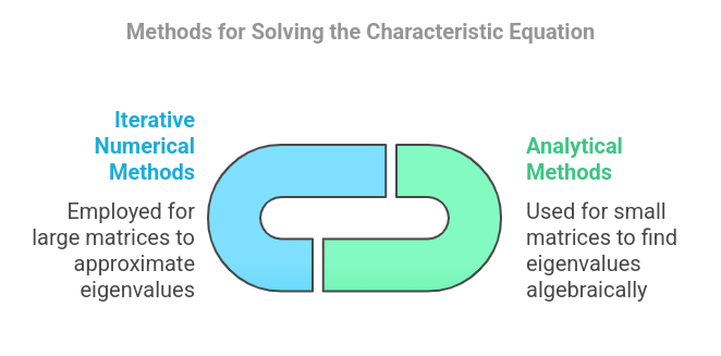
1. Analytical Methods (For Small Matrices)

For small matrices (2×2 or 3×3), eigenvalues can be found algebraically by solving the determinant equation manually.

For a 2×2 matrix, given:

A=[abcd]A = \begin{bmatrix} a & b \\ c & d \end{bmatrix}A=[ac​bd​]
The characteristic equation:
∣a−λbcd−λ∣=0\begin{vmatrix} a - \lambda & b \\ c & d - \lambda \end{vmatrix} = 0​a−λc​bd−λ​​=0

Expands to:

(a−λ)(d−λ)−bc=0(a - \lambda)(d - \lambda) - bc = 0(a−λ)(d−λ)−bc=0
Solving this quadratic equation gives the eigenvalues.

For a 3×3 matrix, the determinant expands into a cubic equation, which can still be solved analytically but is more complex.

2. Iterative Numerical Methods (For Large Matrices)

For large matrices, solving the characteristic polynomial explicitly is inefficient due to numerical instability and computational cost. Instead, iterative algorithms are used to approximate eigenvalues.

Numerical Techniques and Common Algorithms

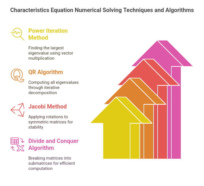
1. Power Iteration Method

• Used to find the largest eigenvalue.
• Starts with a random vector and repeatedly multiplies it by the matrix, normalizing at each step.
• Converges to the dominant eigenvector-eigenvalue pair.

Algorithm:

1. Choose a random vector v0v_0v0​.
2. Compute vk+1=Avk∣∣Avk∣∣v_{k+1} = \frac{A v_k}{||A v_k||}vk+1​=∣∣Avk​∣∣Avk​​ repeatedly.
3. The corresponding eigenvalue is approximated by: λ=vkTAvkvkTvk\lambda = \frac{v_k^T A v_k}{v_k^T v_k}λ=vkT​vk​vkT​Avk​​

Pros: Simple, efficient for dominant eigenvalues.
Cons: It does not compute all eigenvalues.

2. QR Algorithm

• Computes all eigenvalues of a matrix by iteratively factorizing it into QR decomposition.
• Given A=QRA = QRA=QR (where QQQ is an orthogonal matrix and RRR is upper triangular), the process iteratively updates AkA_kAk​ as:
  Ak+1=RkQkA_{k+1} = R_k Q_kAk+1​=Rk​Qk​
• Converges to an upper triangular matrix where diagonal elements are the eigenvalues.

Pros: Works well for dense matrices.
Cons: Computationally expensive for very large matrices.

3. Jacobi Method (For Symmetric Matrices)

• Used when AAA is symmetric, where eigenvalues correspond to diagonal elements after rotation.
• Applies successive Givens rotations to reduce off-diagonal elements iteratively.

Pros: More stable for symmetric matrices.
Cons: Slower than QR for large matrices.

4. Divide and Conquer Algorithm

• Breaks a matrix into smaller submatrices, computes eigenvalues separately, and merges results.
• Used in optimized implementations like LAPACK (Linear Algebra PACKage).

Pros: Faster for large sparse matrices.
Cons: Requires extra memory.

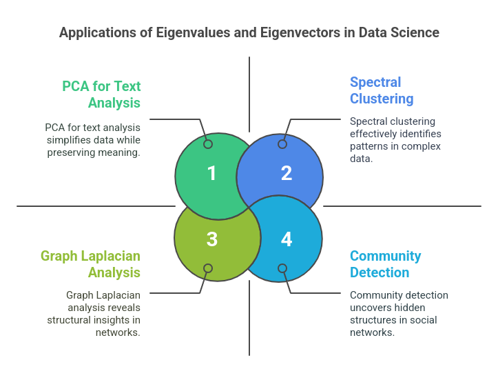
Applications of the Characteristic Equation in Data Science

Eigenvalues and eigenvectors, derived from solving the characteristic equation, play a crucial role in various data science applications. They are used for dimensionality reduction, clustering, network analysis, and even natural language processing. Here’s how they contribute across different domains:

1. Dimensionality Reduction

Role in Principal Component Analysis (PCA)

Principal Component Analysis (PCA) is one of the most popular techniques for reducing the dimensionality of large datasets while retaining as much information as possible.

• Eigenvalues and eigenvectors of the covariance matrix of the dataset determine the principal components.
• The largest eigenvalues correspond to the most significant principal components, capturing the maximum variance.
• The dataset is projected onto the eigenvectors (principal components), reducing redundancy while preserving meaningful structure.

Mathematical Formulation in PCA

1. Compute the covariance matrix of the dataset XXX: C=1nXTXC = \frac{1}{n} X^T XC=n1​XTX
2. Solve the characteristic equation for eigenvalues λ\lambdaλ and eigenvectors vvv: ∣C−λI∣=0|C – \lambda I| = 0∣C−λI∣=0
3. Select the top k eigenvectors (corresponding to the largest eigenvalues).
4. Project the data onto the selected eigenvectors to get lower-dimensional representations.

Interpreting Eigenvalues to Assess Variance

• Larger eigenvalues indicate dimensions with higher variance (more important features).
• Smaller eigenvalues correspond to dimensions with low variance (less significant features).
• Explained variance ratio helps determine how many principal components are needed.

Example using Python (PCA with Scikit-Learn):

from sklearn.decomposition import PCA
import numpy as np

# Sample dataset
data = np.array([[2, 4], [3, 6], [4, 8], [5, 10]])

pca = PCA(n_components=1)
pca.fit(data)

print("Eigenvalues (Explained Variance):", pca.explained_variance_)
print("Eigenvectors (Principal Components):\n", pca.components_)

PCA is widely used in computer vision, text analysis, and bioinformatics for handling high-dimensional data.

2. Clustering and Spectral Methods

Using Eigen Decomposition in Clustering Algorithms

Eigenvalues play a critical role in spectral clustering, a method that leverages eigenvectors of similarity graphs to detect clusters.

• Traditional clustering (e.g., k-means) struggles with non-linearly separable data.
• Spectral clustering transforms data into a lower-dimensional space using eigenvectors of a similarity matrix (Laplacian matrix).
• The transformed data is then clustered using standard methods like k-means.

Steps in Spectral Clustering:

1. Construct the similarity graph and compute its adjacency matrix AAA.
2. Compute the Laplacian matrix: L=D−AL = D – AL=D−A where DDD is the degree matrix.
3. Compute eigenvalues and eigenvectors of LLL.
4. Use k smallest eigenvectors to represent data in a lower-dimensional space.
5. Apply k-means clustering on the new representation.

Example: Spectral Clustering using Scikit-Learn

from sklearn.cluster import SpectralClustering

# Define spectral clustering model
spectral = SpectralClustering(n_clusters=2, affinity='nearest_neighbors', random_state=42)

# Fit model on data
labels = spectral.fit_predict(data)

Spectral clustering is widely used in community detection, image segmentation, and anomaly detection.

3. Graph and Network Analysis

Spectral Graph Theory and Its Applications

Eigenvalues and eigenvectors are fundamental in graph theory, where they are used to analyze network structures.

• The Laplacian matrix LLL encodes important graph properties.
• The smallest nonzero eigenvalue (called the Fiedler value) determines graph connectivity.
• Eigenvector centrality measures the importance of nodes in a network (e.g., Google’s PageRank algorithm).

Applications:

• Community detection: Clustering nodes into groups.
• Social network analysis: Identifying influential users.
• Anomaly detection: Finding unusual connections in a graph.

Example: Computing Eigenvalues of a Graph Laplacian in NetworkX

import networkx as nx
import numpy as np
from scipy.linalg import eigvals

# Create a simple graph
G = nx.karate_club_graph()
L = nx.laplacian_matrix(G).toarray()

# Compute eigenvalues of Laplacian matrix
eigenvalues = eigvals(L)

print("Graph Laplacian Eigenvalues:", eigenvalues)

Spectral methods in graph analysis are essential for applications like fraud detection, cybersecurity, and recommendation systems.

4. Other Applications in Data Science

Eigenvalues and eigenvectors have broader applications across various fields:

Natural Language Processing (NLP)

• Latent Semantic Analysis (LSA): Uses Singular Value Decomposition (SVD) (which is closely related to eigen decomposition) to extract hidden topics in text data.
• Word embeddings: Eigen decomposition helps understand word relationships in NLP.

Example: Topic Modeling with LSA

from sklearn.decomposition import TruncatedSVD
from sklearn.feature_extraction.text import TfidfVectorizer

documents = ["Machine learning is amazing",
             "Deep learning improves AI",
             "Data science is evolving rapidly"]

vectorizer = TfidfVectorizer()
X = vectorizer.fit_transform(documents)

lsa = TruncatedSVD(n_components=2)
lsa.fit(X)

print("Singular values:", lsa.singular_values_)

Image Processing

• Eigenfaces in facial recognition: Eigenvalue decomposition is used to reduce image data while preserving key features.
• PCA in image compression: Compresses images by keeping only significant eigenvalues.

Example: PCA for Image Compression

from sklearn.decomposition import PCA
from skimage import io

image = io.imread('sample_image.jpg', as_gray=True)
pca = PCA(n_components=50)  # Keep only 50 principal components
compressed_image = pca.inverse_transform(pca.fit_transform(image))

Recommendation Systems

• Matrix Factorization (SVD): Used in collaborative filtering models for personalized recommendations (e.g., Netflix, Amazon).
• Low-rank approximations: Reduce noise in rating matrices.

Example: SVD for Recommendations

from scipy.sparse.linalg import svds
import numpy as np

# Sample user-item matrix
R = np.array([[5, 3, 0, 1],
              [4, 0, 0, 1],
              [1, 1, 0, 5]])

U, sigma, Vt = svds(R, k=2)  # Compute low-rank approximation

This approach improves recommendation quality by capturing user preferences efficiently.

Challenges and Considerations

While eigenvalues and eigenvectors play a crucial role in various data science applications, solving the characteristic equation and applying eigen decomposition come with computational and theoretical challenges. Below are key considerations:

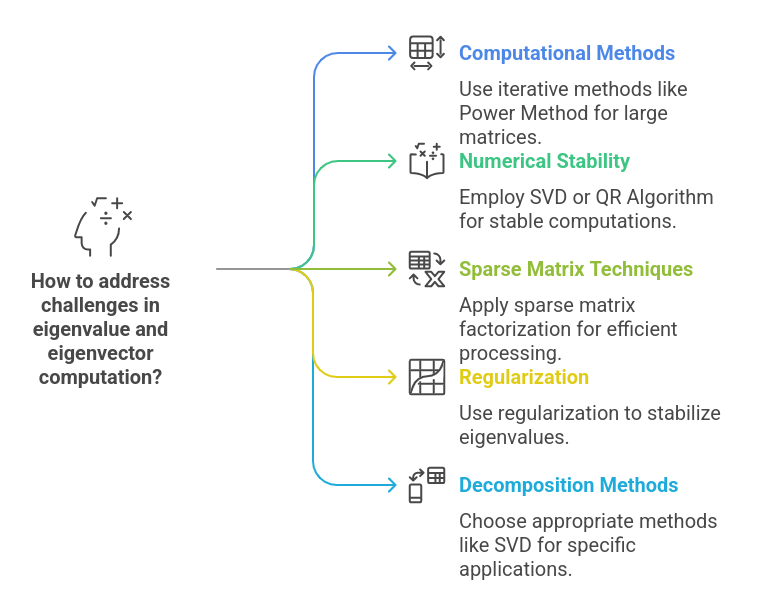
1. Computational Challenges

High-Dimensional Matrices

• In real-world data science problems, matrices can be very large (e.g., 1000×1000 or more), making direct computation of eigenvalues computationally expensive.

• Solution: Use iterative methods like the Power Method or Lanczos Algorithm to compute dominant eigenvalues efficiently.

Numerical Stability Issues

• Eigenvalue computations involve floating-point arithmetic, which can lead to rounding errors.

• Solution: Use Singular Value Decomposition (SVD) or QR Algorithm, which are more stable than direct determinant calculations.

Sparse Matrices

• Many applications involve sparse matrices (e.g., Graph Theory, NLP), where most values are zero.

• Solution: Use sparse matrix factorization techniques like ARPACK (for eigen decomposition) or Scipy’s sparse.linalg.eigs() for efficient computation.

2. Theoretical Considerations

Eigenvalue Sensitivity

• Small perturbations in data can significantly alter eigenvalues. This is crucial in PCA, where small changes in the dataset can impact the principal components.

• Solution: Use regularization techniques to stabilize eigenvalues, especially in machine learning applications.

Interpreting Eigenvalues in Data Science

• Not all eigenvalues have clear interpretations in certain applications. For example, in PCA, choosing how many principal components to retain requires setting a variance threshold.

• Solution: Use the Kaiser criterion (retain eigenvalues > 1) or screen plot analysis to determine the number of components.

3. Algorithmic Trade-offs

Exact vs. Approximate Solutions

• Finding exact eigenvalues for large matrices is computationally expensive.
• Solution: Many real-world applications use approximate methods like the Power Method for fast computation.

Choice of Decomposition Method

• Different applications require different decomposition methods (e.g., eigen decomposition vs. SVD).
• Example:
  • PCA uses eigen decomposition on the covariance matrix.
  • Recommendation systems prefer SVD for handling missing values in data.

4. Domain-Specific Challenges

Graph and Network Analysis

• Computing eigenvalues for large graphs (e.g., social networks) is complex. Spectral clustering methods rely on the eigenvalues of the Laplacian matrix, which can be slow to compute.
• Solution: Use approximate eigen decomposition methods for large-scale graphs.

Deep Learning and Neural Networks

• Eigenvalues can help analyze weight matrices in deep learning, but computing them for deep networks is difficult due to high dimensionality.
• Solution: Use batch-wise matrix approximations for efficient computation.

Conclusion

The characteristic equation, eigenvalues, and eigenvectors are fundamental to many data science applications, from dimensionality reduction (PCA) and clustering to graph analytics and deep learning. 

However, their practical use comes with computational challenges, requiring efficient numerical techniques and algorithmic optimizations. Mastering these concepts is crucial for tackling real-world machine learning and AI problems. 

If you’re looking to deepen your understanding of linear algebra, eigen decomposition, and their applications in data science, consider enrolling in MIT’s Data Science and Machine Learning course in collaboration with Great Learning, designed to equip you with hands-on skills and industry-relevant expertise.