In this article, we will find out why we cannot train Recurrent Neural networks with the regular backpropagation and use its modified version known as the backpropagation through time.
What is backpropagation?
First, let us briefly go over backpropagation, Backpropagation is a training algorithm that is used for training neural networks. When training a neural network, we are actually tuning the weights of the network to minimize the error with respect to the already available true values(labels) by using the Backpropagation algorithm. It is a supervised learning algorithm as we find errors with respect to already given labels. The general algorithm is as follows:
- Present a training input pattern and propagate it through the network to get an output.
- Compare the predicted outputs to the expected outputs and calculate the error.
- Calculate the derivatives of the error with respect to the network weights.
- Use these calculated derivatives to adjust the weights to minimize the error.
- Repeat.
Unrolling the RNN(recurrent neural network)
Here I am only going to briefly discuss RNN, enough to understand how the backpropagation algorithm is applied to recurrent neural network or RNN. You can click here to get a detailed article about RNN(recurrent neural network). So as you might know RNN is used to work with sequential data and in sequential data, there is a lot of information present in the data as well as in the sequence of the data. So in RNN, we have these loops that allow information to persist through time.
Take a look at the architecture of RNN below:
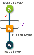
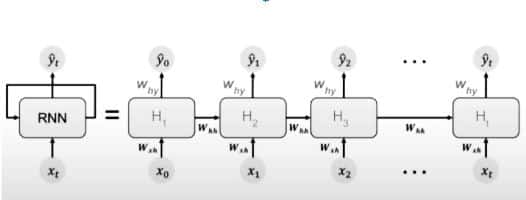
Let us understand what happens by unfolding the above figure:
.
So now that we unfolded the RNN with loop, we got the above figure. At time =t0 , we input x0 to our network and we get an output y0 , at time =t1 , we input x1 to our network and we get an output y1, Now as you can see the figure, to calculate output the network uses input x and the cell state from the previous timestamp.To calculate certain Hidden state here is the formula
We usually use tanh activation, but you can use anyone more suitable. And to calculate the output at each step, here is the formula
Now to calculate the error, we just take the output and calculate its error with respect to the label(real output), but here we have multiple outputs, one at each time stamp and thus the regular backpropagation is not suitable here. Thus we modify this algorithm and call the new algorithm as backpropagation through time.
Note: It is important to remember that the value of Whh ,Wxh and Why does not change across the timestamps, which means that for all inputs in a sequence, the values of these weights is same.
Backpropagation through time
Now the questions that should come to your mind are
- What is the total loss for this network?
- How do we update the weights Whh ,Wxh and Why?
The total loss is simply the sum of the losses overall timestamps.For example,in the figure below,En is the loss at each time stamp and instead of h to denote cell state, I am using s here.
Then total loss = E0 + E1 + E2 + E4
In general, we can say the total error is equal to summation over all the errors across timestamps t,
Where Et(yt,yt) is the error made at timestamp t.
Now we have to calculate the gradient of this loss with respect to Whh ,Wxh and Why.For simplicity I am going to denote Whh as W,Wxh as U and Why .as V.
It is quite easy to calculate the derivative of loss with respect to V as it only depends on the values at the current time step. But when it comes to calculating the derivative of loss with respect to W and U, it becomes a bit tricky.

As you can see the first part of this equation,i.e derivative of E w.r.t s4 can be easily calculated as it only depends on V.But to calculate the derivative of s4 with respect to W is not so easy.
The value of s4depends on s3 which itself is a function W, therefore we cannot calculate the derivative of s4 keeping s3 as constant. In such networks, the derivative has two parts, implicit and explicit. In explicit part, we assume all other inputs as constant whereas in implicit part we sum over all the indirect paths. Therefore we calculate the derivative as :
Now we can easily put this value in the previous formula to calculate the derivative of E with respect to W. In a similar manner, you can also calculate the derivative of E with respect to U.Now that we have all the three derivatives, we can easily update our weights. This algorithm is called backpropagation through time or BPTT for short as we used values across all the timestamps to calculate the gradients.
It is very difficult to understand these derivations in text, here is a good explanation of this derivation
Limitations of backpropagation through time :
When using BPTT(backpropagation through time) in RNN, we generally encounter problems such as exploding gradient and vanishing gradient.
To avoid exploding gradient, we simply use a method called gradient clipping where at each timestamp, we can check if the gradient > threshold and if it is, we normalize it. This helps to tackle exploding gradient. To tackle the vanishing gradient problem these are the possible solutions:
- Use ReLU instead of tanh or sigmoid activation function.
- Proper initialization of the W matrix can reduce the effect of vanishing gradients. It has been seen that initializing with an identity matrix helps in tackling this problem.
- Using gated cells such as LSTM or GRUs
This brings us to the end of this article where we learned how we update weights in RNN by using Backpropagation through time. To know more about Machine learning and get a free course, click the banner below:
